案例五 蛋白-配体相互作用
本文以gromacs官方教程五的内容为基础,将指导用户完成设置模拟系统的过程,该系统包含蛋白质-配体的复合物。通过教程将学习到动力学模拟及数据分析的全流程操作。

准备文件
分子对接一般负责寻找小分子配体和大分子受体的某个相互结合位点,相当于单帧图片;而动力学模拟则是在此基础上计算模拟配体-受体的动态相互作用过程,因此,动力学模拟往往是在分子对接完成后,对对接复合物进行操作的。
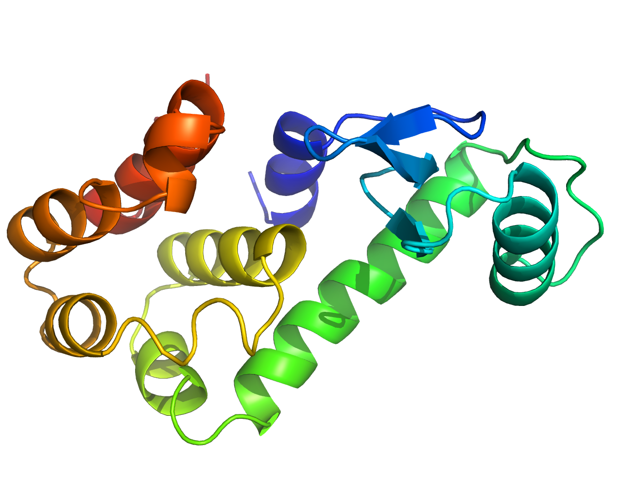
这里的示例大蛋白选用3HTB蛋白,在RCSB数据库中下载蛋白文件3THB,提前将蛋白质进行加氢、去水、去配体操作,在日常操作中,最好选择使用分子对接后的大蛋白和小分子,分别为PDB和MOL2文件。
建议工作中蛋白质统一命名为protein.pdb,小分子统一命名为mol.mol2
本教程的所有蛋白、配体文件以及所需的五种参数配置文件可点击此处下载
大分子准备
使用以下命令选择力场,构建蛋白质拓扑:
gmx pdb2gmx -f protein.pdb -o protein.gro -ter对于输出的下列待选项目,我们需要选择力场和水模型,力场选择AMBER99SB-ILDN,水模型选择TIP3P
From '/usr/local/gromacs/share/gromacs/top':
 2: AMBER03 protein, nucleic AMBER94 (Duan et al., J. Comp. Chem. 24, 1999-2012, 2003)
 3: AMBER94 force field (Cornell et al., JACS 117, 5179-5197, 1995)
 4: AMBER96 protein, nucleic AMBER94 (Kollman et al., Acc. Chem. Res. 29, 461-469, 1996)
 5: AMBER99 protein, nucleic AMBER94 (Wang et al., J. Comp. Chem. 21, 1049-1074, 2000)
 6: AMBER99SB protein, nucleic AMBER94 (Hornak et al., Proteins 65, 712-725, 2006)
 7: AMBER99SB-ILDN protein, nucleic AMBER94 (Lindorff-Larsen et al., Proteins 78, 1950-58, 2010)
 8: AMBERGS force field (Garcia & Sanbonmatsu, PNAS 99, 2782-2787, 2002)
 9: CHARMM27 all-atom force field (CHARM22 plus CMAP for proteins)
10: GROMOS96 43a1 force field
11: GROMOS96 43a2 force field (improved alkane dihedrals)
12: GROMOS96 45a3 force field (Schuler JCC 2001 22 1205)
13: GROMOS96 53a5 force field (JCC 2004 vol 25 pag 1656)
14: GROMOS96 53a6 force field (JCC 2004 vol 25 pag 1656)
15: GROMOS96 54a7 force field (Eur. Biophys. J. (2011), 40,, 843-856, DOI: 10.1007/s00249-011-0700-9)
16: OPLS-AA/L all-atom force field (2001 aminoacid dihedrals)在此过程中可能会报错,提示H原子类型不匹配或氢原子命名错误,这时可以选择使用-ignh命令,忽视原有氢原子,此时gromacs会自动加全氢
gmx pdb2gmx -f protein.pdb -o protein.gro -ter -ignh在这一步里可能会出现Total charge in system x.000 e的提示,说明体系电荷不为零,在后续的溶剂化过程中为其添加抗衡离子即可。
最终会生成拓topol.top拓扑文件,和大蛋白的protein.gro文件,该文件可以用pymol可视化预览。
小分子准备
上步中拆分的小分子配体保存为MOL2格式,如果是PDB格式,则需要将其转化为MOL2格式,得到一个mol.mol2文件。
该文件只包含一个小分子,可以利用Pymol为其加氢,同时将@<TRIPOS>MOLECULE下的名称改为MOL,或其他统一名称,作为该配体的名称,同时确保ATOM列的MOL与该名称一致即可。
@<TRIPOS>MOLECULE
MOL
22 22 1
SMALL
USER_CHARGES
@<TRIPOS>ATOM
1	 OAB	23.412	-23.536	-4.342	O.3	1	MOL1	0.000
2	  C4	24.294	-24.124	-0.071	C.3	1	MOL1	0.000
3	  C7	21.553	-27.214	-4.112	C.2	1	MOL1	0.000
4	  C8	22.068	-26.747	-5.331	C.2	1	MOL1	0.000
5	  C9	22.671	-25.512	-5.448	C.2	1	MOL1	0.000
6	 C10	22.769	-24.730	-4.295	C.2	1	MOL1	0.000
7	 C11	21.693	-26.459	-2.954	C.2	1	MOL1	0.000
8	 C12	22.294	-25.187	-3.075	C.2	1	MOL1	0.000
9	 C13	22.463	-24.414	-1.808	C.3	1	MOL1	0.000
10	 C14	23.925	-24.704	-1.394	C.3	1	MOL1	0.000
11	 H01	23.560	-23.216	-3.449	 H	1	MOL1	0.000
12	 H02	25.135	-23.442	-0.196	 H	1	MOL1	0.000
13	 H03	23.443	-23.579	0.337	 H	1	MOL1	0.000
14	 H04	24.575	-24.926	0.612	 H	1	MOL1	0.000
15	 H05	21.040	-28.175	-4.073	 H	1	MOL1	0.000
16	 H06	21.989	-27.381	-6.214	 H	1	MOL1	0.000
17	 H07	23.057	-25.160	-6.405	 H	1	MOL1	0.000
18	 H08	21.352	-26.834	-1.989	 H	1	MOL1	0.000
19	 H09	21.743	-24.698	-1.041	 H	1	MOL1	0.000
20	 H10	22.311	-23.348	-1.979	 H	1	MOL1	0.000
21	 H11	24.026	-25.786	-1.309	 H	1	MOL1	0.000
22	 H12	24.588	-24.287	-2.152	 H	1	MOL1	0.000
@<TRIPOS>BOND
1 1 6 1
2 1 11 1
3 2 10 1
4 2 12 1
5 2 13 1
6 2 14 1
7 3 4 ar
8 3 7 ar
9 3 15 1
10 4 5 ar
11 4 16 1
12 5 6 ar
13 5 17 1
14 6 8 ar
15 7 8 ar
16 7 18 1
17 8 9 1
18 9 10 1
19 9 19 1
20 9 20 1
21 10 21 1
22 10 22 1该小分子mol2文件(邻丙基苯酚)可用pymol预览如下: 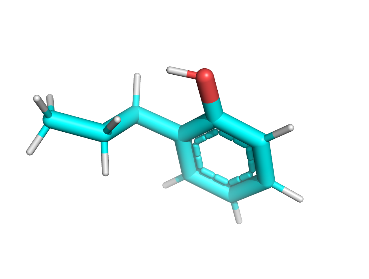
小分子力场的选择是一个非常复杂的过程,还涉及多个软件配合,这里我们可以使用计算化学公社卢天老师开发的sobtop软件(点击此处下载),快速构建小分子拓扑具体步骤如下:
- 打开sobtop,把小分子mol.mol2拖入sobtop
- //选择1,生成top文件
- //选择3,尽可能使用GAFF力场
- //选择0,进入下一步
- //选择4,如果可能,预先构建成键参数,任意猜测缺少的选项
- //回车,生成的top文件生成在sobtop软件根目录下
- //回车,生成的itp位置限制文件在sobtop软件根目录下
- //选择2,生成gro文件
- //回车,生成的gro文件在sobtop软件根目录下
- //回车,退出sobtop软件
这时sobtop工作路径会出现mol.gro、mol.itp、mol.top三个文件,这就是小分子的拓扑文件,把他们复制到模拟的路径即可。
构建复合体
合并文件
新建一个complex.gro文件,先将3HTB_processed.gro的内容复制进去,再把sobtop生成的小分子mol.gro的以下内容复制进去,并规整文件。
更新总的原子数目,增加 complex.gro 的第二行,即原有大蛋白的原子数加上添加进来的小分子原子数,注意该文件不能有空行的出现:
Gyas ROwers Mature At Cryogenic Speed
2614+22=2636修改后的complex.gro文件如下:
  163ASN    OC1 2613   0.566  -0.780  -0.053
  163ASN    OC2 2614   0.624  -0.616  -0.140
    1MOL    OAB    1   2.341  -2.354  -0.434
    1MOL     C4    2   2.429  -2.412  -0.007
    1MOL     C7    3   2.155  -2.721  -0.411
    1MOL     C8    4   2.207  -2.675  -0.533
    1MOL     C9    5   2.267  -2.551  -0.545
    1MOL    C10    6   2.277  -2.473  -0.429
    1MOL    C11    7   2.169  -2.646  -0.295
    1MOL    C12    8   2.229  -2.519  -0.307
    1MOL    C13    9   2.246  -2.441  -0.181
    1MOL    C14   10   2.393  -2.470  -0.139
    1MOL    H01   11   2.356  -2.322  -0.345
    1MOL    H02   12   2.514  -2.344  -0.020
    1MOL    H03   13   2.344  -2.358   0.034
    1MOL    H04   14   2.458  -2.493   0.061
    1MOL    H05   15   2.104  -2.817  -0.407
    1MOL    H06   16   2.199  -2.738  -0.621
    1MOL    H07   17   2.306  -2.516  -0.641
    1MOL    H08   18   2.135  -2.683  -0.199
    1MOL    H09   19   2.174  -2.470  -0.104
    1MOL    H10   20   2.231  -2.335  -0.198
    1MOL    H11   21   2.403  -2.579  -0.131
    1MOL    H12   22   2.459  -2.429  -0.215
5.99500 5.19182 9.66100 0.00000 0.00000 -2.99750 0.00000 0.00000 0.00000添加完成后,可以使用pymol可视化观察complex.gro,应该可以看到大蛋白和小分子配体共存。 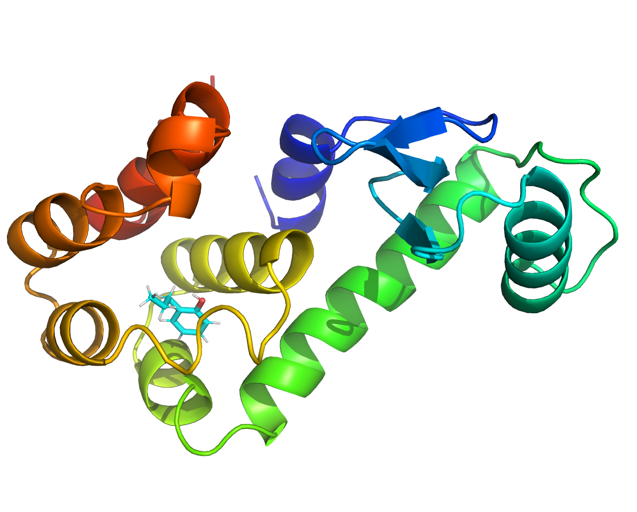
构建拓扑
蛋白质的限制势itp文件在pdb2gmx的时候已经产生,但小分子的没有,genrestr是对输入的结构产生坐标或距离限制势itp文件(posre_mol.itp)的工具,接下来运行命令,进行限制势的产生:
gmx genrestr -f mol.gro -o posre_mol.itp选择组0,system默认的位置限制势常数是
Reading structure file
Select group to position restrain
Group     0 (         System) has    22 elements
Group     1 (          Other) has    22 elements
Group 2 ( MOL) has 22 elements得到了小分子的位置限制文件posre_mol.itp,将下列语句插入到mol.itp文件的末尾,复制时连同“#”井号一同复制,最好在末尾添加之前空一行,方便检查文件错误。
#ifdef POSRES
#include "posre_mol.itp"
#endif最终修改好的mol.itp文件末尾应该为如下内容:
[ dihedrals ] ; impropers
; atom_i  atom_j  atom_k  atom_l  functype  phase (Deg.)  kd (kJ/mol)  pn
    4       7       3      15         4       180.000       4.60240    2     ; C8-C11-C7-H05, prebuilt X-X-ca-ha
    3       5       4      16         4       180.000       4.60240    2     ; C7-C9-C8-H06, prebuilt X-X-ca-ha
    4       6       5      17         4       180.000       4.60240    2     ; C8-C10-C9-H07, prebuilt X-X-ca-ha
    1       5       6       8         4       180.000       4.60240    2     ; OAB-C9-C10-C12, guess (same as GAFF X -X -ca-ha)
    3       8       7      18         4       180.000       4.60240    2     ; C7-C12-C11-H08, prebuilt X-X-ca-ha
    6       7       8       9         4       180.000       4.60240    2     ; C10-C11-C12-C13, prebuilt ca-ca-ca-c3

#ifdef POSRES
#include "posre_mol.itp"
#endif这样当mdp中使用define = -DPOSRES的时候配体的位置也会被限制。
把配体的itp文件引入整体的拓扑文件topol.top,在引入的时候需要将小分子的mol.itp文件引入到蛋白质链之前,因为mol.itp最开头定义了[atomtypes]因此,这个itp要最优先被引入。
即,将下列黄色语句插入到引入蛋白质的topol.itp文件引入之前,最终顺序如下;
; Include forcefield parameters
#include "amber99sb-ildn.ff/forcefield.itp"

#include "mol.itp"

[ moleculetype ]
; Name            nrexcl
Protein_chain_A 3在末尾的[molecules]中引入MOL 1,将topol.top的格式与complex.gro中分子出现的顺序对应:
[ molecules ]
; Compound        #mols
Protein_chain_A     1
MOL                 1
溶剂化
设置盒子
使用以下命令设置模拟盒子,这里选用立方体盒子,可能会增加计算量,但是不容易产生边界相互作用的问题:
gmx editconf -f complex.gro -o complex_box.gro -d 0.8 -bt cubic也可以选择三斜晶胞盒子:
gmx editconf -f complex.gro -o complex_box.gro -bt dodecahedron -d 1.0加溶剂
得到complex_box.gro文件后为容器内加水:
gmx solvate -cp complex_box.gro -cs spc216.gro -o complex_SOL.gro -p topol.top这里的-cs spc216.gro可以不写,意思是默认选择GROMACS内置的预平衡的SPC水模型(216个水分子构成的立方盒子),默认是简单点电荷(SPC)水模型。其他可选溶剂如tip3p.gro、tip4p.gro等。
注意这一步加水后有可能topol.top文件最后一行的SOL可能会串行,需要手动添加回车,避免其与mol 1连在同一行,容易在后续处理中报错。
这一步完成后的topol.itp文件末尾会增加数万个水分子:
[ molecules ]
; Compound        #mols
Protein_chain_A     1
MOL                 1
SOL 12750最终得到的complex_SOL.gro文件可用pymol预览: 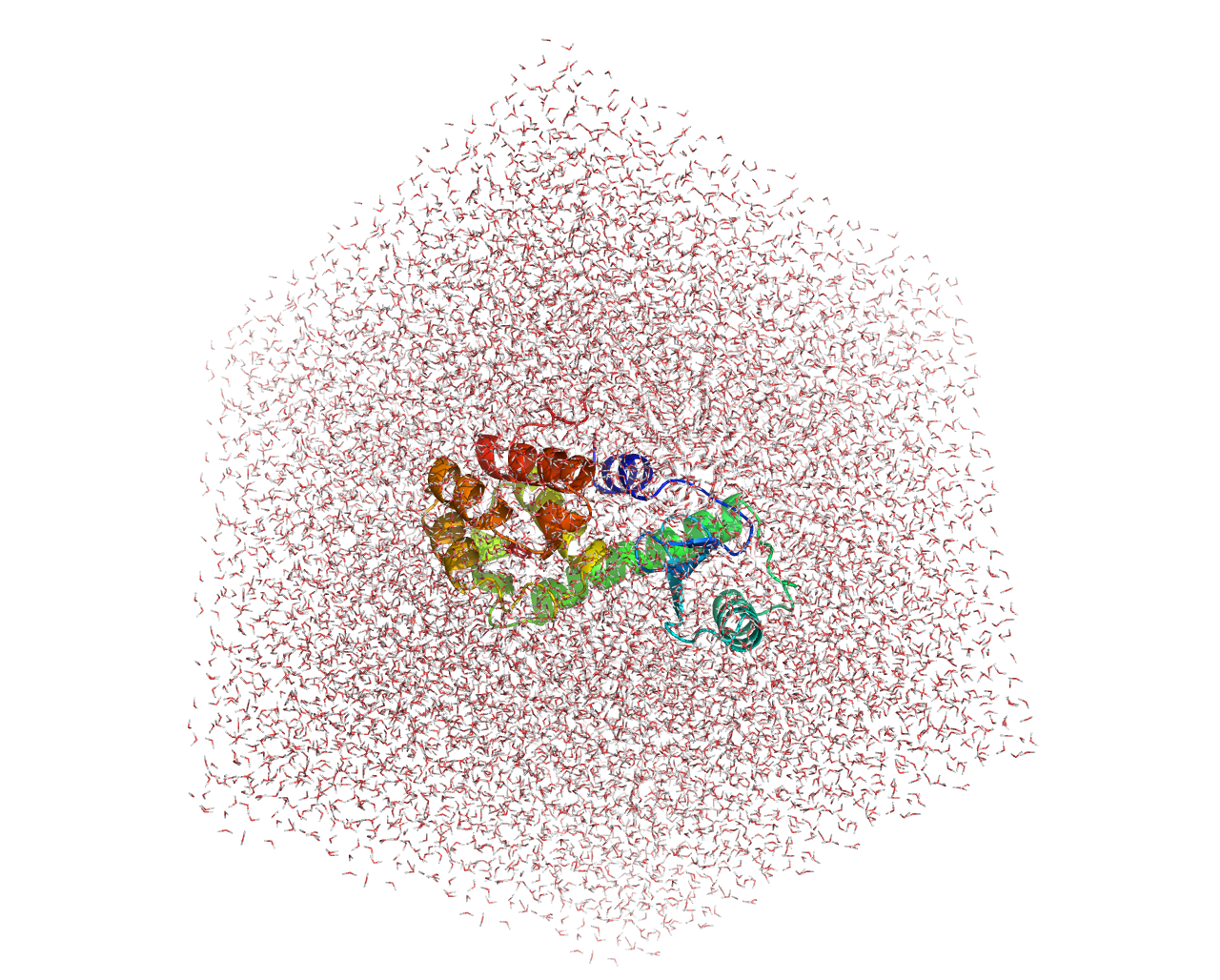
添加中和离子
构建一个ions.mdp配置文件:
; LINES STARTING WITH ';' ARE COMMENTS
title		    = Minimization	; Title of run

; Parameters describing what to do, when to stop and what to save
integrator	    = steep		; Algorithm (steep = steepest descent minimization)
emtol		    = 1000.0  	; Stop minimization when the maximum force < 10.0 kJ/mol
emstep          = 0.01      ; Energy step size
nsteps		    = 50000	  	; Maximum number of (minimization) steps to perform

; Parameters describing how to find the neighbors of each atom and how to calculate the interactions
nstlist		    = 1		    ; Frequency to update the neighbor list and long range forces
cutoff-scheme   = Verlet
ns_type		    = grid		; Method to determine neighbor list (simple, grid)
rlist		    = 1.0		; Cut-off for making neighbor list (short range forces)
coulombtype	    = cutoff	; Treatment of long range electrostatic interactions
rcoulomb	    = 1.0		; long range electrostatic cut-off
rvdw		    = 1.0		; long range Van der Waals cut-off
pbc             = xyz 		; Periodic Boundary Conditions
生成临时tpr文件:
gmx grompp -f ions.mdp -c complex_SOL.gro -p topol.top -o ions.tpr -maxwarn 1这里如果警告较多可以将maxwarn的数值改大一些。
最后为体系加离子,使得整个体系变为电中性:
gmx genion -s ions.tpr -p topol.top -o system.gro -neutral这里选择分组时选择 SOL(15) 对应的分组,产生的带有离子且电中性的体系为system.gro。同时可以额外使用-pname NA -nname CL来选择添加的阴阳离子类型,具体名称根据力场来选择。
最终的结果为总拓扑文件[ molecules ]后出现对应数目的离子,同时使用pymol也观察到system.gro文件中加载了氯离子,离子数目应该和上文的电荷数Total charge in system x.000 e相对应:
[ molecules ]
; Compound        #mols
Protein_chain_A     1
MOL                 1
SOL             12744
CL 6最终得到的system.gro文件可以用pymol预览,看到已经成功添加了6个氯离子: 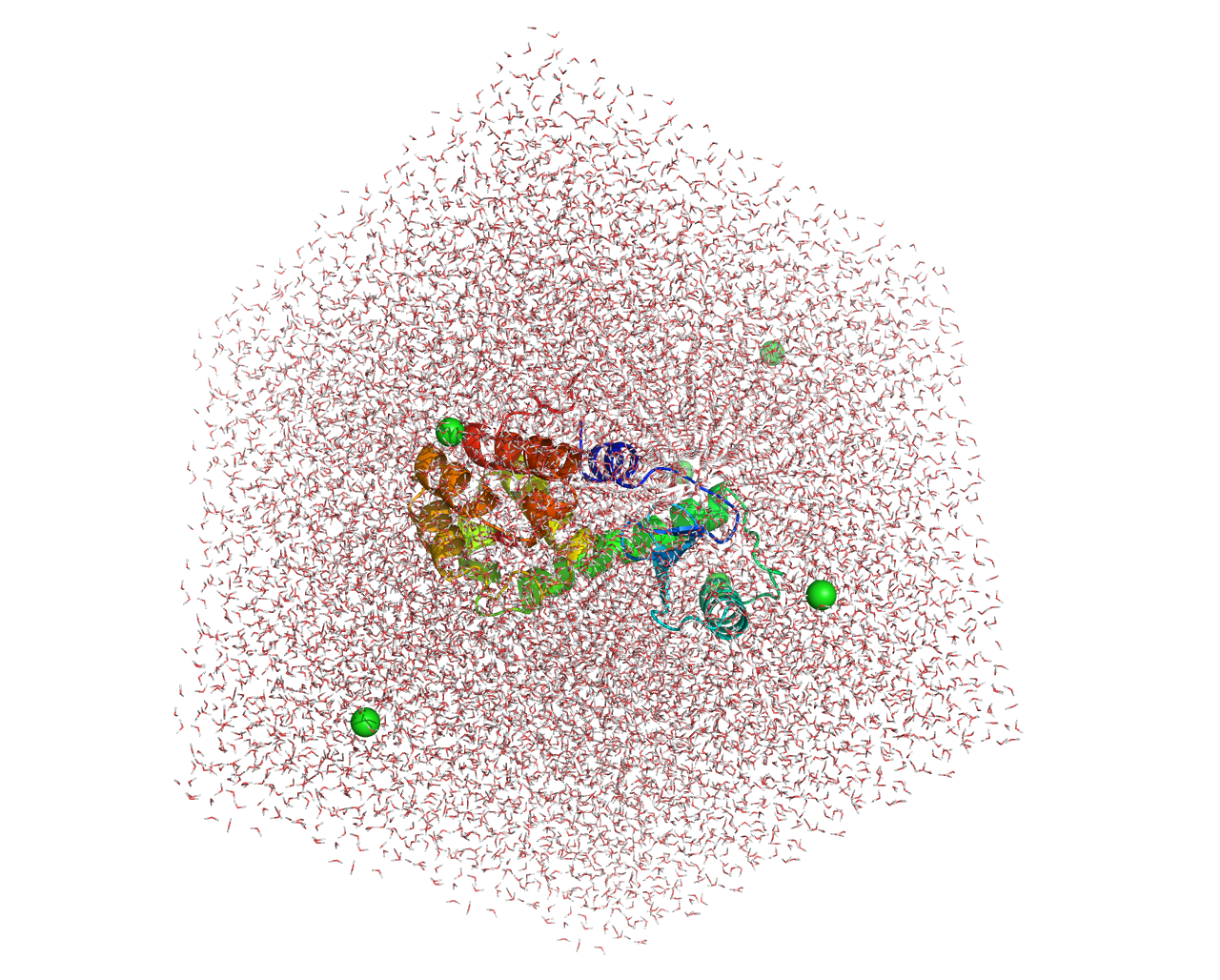
能量最小化
创建如下em.mdp文件:
; LINES STARTING WITH ';' ARE COMMENTS
title		    = Minimization	; Title of run

; Parameters describing what to do, when to stop and what to save
integrator	    = steep		; Algorithm (steep = steepest descent minimization)
emtol		    = 1000.0  	; Stop minimization when the maximum force < 10.0 kJ/mol
emstep          = 0.01      ; Energy step size
nsteps		    = 50000	  	; Maximum number of (minimization) steps to perform

; Parameters describing how to find the neighbors of each atom and how to calculate the interactions
nstlist		    = 1		        ; Frequency to update the neighbor list and long range forces
cutoff-scheme   = Verlet
ns_type		    = grid		    ; Method to determine neighbor list (simple, grid)
rlist		    = 1.2		    ; Cut-off for making neighbor list (short range forces)
coulombtype	    = PME		    ; Treatment of long range electrostatic interactions
rcoulomb	    = 1.2		    ; long range electrostatic cut-off
vdwtype         = cutoff
vdw-modifier    = force-switch
rvdw-switch     = 1.0
rvdw		    = 1.2		    ; long range Van der Waals cut-off
pbc             = xyz 		    ; Periodic Boundary Conditions
DispCorr = no使用以下命令载入em.mdp文件,开始能量最小化:
gmx grompp -f em.mdp -c system.gro -p topol.top -o em.tpr使用启动能量最小化:
gmx mdrun -v -deffnm em最终的系统收敛会输出以下内容:
Steepest Descents converged to Fmax < 1000 in 143 steps
Potential Energy  = -4.9014547e+05
Maximum force     =  8.7411469e+02 on atom 27
Norm of force     =  5.6676244e+01
然后运行该命令,选择 "10 0" (Potential, system) ,可以得到能量最小化曲线,使用看图软件即可查看能量变化图:
gmx energy -f em.edr -o potential.xvg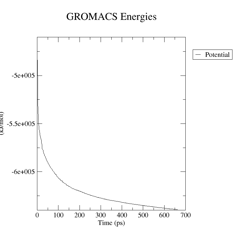
平衡
约束配体
为了约束配体,我们需要为其生成位置约束拓扑。首先,为 MOL 创建一个仅包含其非氢原子的索引组:
gmx make_ndx -f mol.gro -o index_mol.ndx依次输入下列内容:
 > 0 & ! a H*
 > q
然后,执行 genrestr 模块并选择这个新创建的索引组(将是 index_mol.ndx 文件中的第 3 组):
gmx genrestr -f mol.gro -n index_mol.ndx -o posre_mol.itp -fc 1000 1000 1000选择组 3:
Reading structure file
Select group to position restrain
Group     0 (         System) has    22 elements
Group     1 (          Other) has    22 elements
Group     2 (            MOL) has    22 elements
Group 3 ( System_&_!H*) has 10 elements将此信息包含在拓扑中,方法有很多种。最简单的,如果只想在蛋白质也被约束时抑制配体,在指示的位置将以下黄色代码行添加到拓扑文件topol.itp的对应位置中:
; Include Position restraint file
#ifdef POSRES
#include "posre.itp"
#endif

; Ligand position restraints
#ifdef POSRES
#include "posre_mol.itp"
#endif

; Include water topology
#include "amber99sb-ildn.ff/tip3p.itp"

#ifdef POSRES_WATER
位置很重要,必须按照指示在拓扑中调用 posre_mol.itp。
mol.itp 中的参数为我们的配体定义了一个指令,引用文件以包含水拓扑结构 (tip3p.itp) 结束,在其他任何位置调用 posre_mol.itp 将尝试将位置约束参数应用于错误的分子类型。
最后需要一个合并蛋白质和 MOL 的特殊索引组,通过 make_ndx 模块来实现这,提供整个系统的任何坐标文件。这里使用的是 em.gro,这是我们系统的输出(最小化)结构:
gmx make_ndx -f em.gro -o index.ndx将显示以下提示词:
  0 System              : 33506 atoms
  1 Protein             :  2614 atoms
  2 Protein-H           :  1301 atoms
  3 C-alpha             :   163 atoms
  4 Backbone            :   489 atoms
  5 MainChain           :   651 atoms
  6 MainChain+Cb        :   803 atoms
  7 MainChain+H         :   813 atoms
  8 SideChain           :  1801 atoms
  9 SideChain-H         :   650 atoms
 10 Prot-Masses         :  2614 atoms
 11 non-Protein         : 30892 atoms
 12 Other               :    22 atoms
 13 MOL                 :    22 atoms
 14 CL                  :     6 atoms
 15 Water               : 30864 atoms
 16 SOL                 : 30864 atoms
 17 non-Water           :  2642 atoms
 18 Ion                 :     6 atoms
 19 MOL                 :    22 atoms
 20 CL                  :     6 atoms
 21 Water_and_ions      : 30870 atoms
将 “Protein” 和 “MOL” 组与以下内容合并,输入"1 | 13",再输入q退出:
> 1 | 13
> q可以看到输出信息,创建了一个编号为22的索引组:
Copied index group 1 'Protein'
Copied index group 13 'MOL'
Merged two groups with OR: 2614 22 -> 2636

22 Protein_MOL : 2636 atoms该索引组的名称为Protein_MOL,应该确保名称和下面的.mdp文件相对应。
为了确保名称一致,可以使用name命令更改名称,最后输入q,退出:
Copied index group 1 'Protein'
Copied index group 13 'MOL'
Merged two groups with OR: 2614 22 -> 2636

 22 Protein_MOL         :  2636 atoms

> name 22 New_name


> q也可以直接在index.ndx中修改索引组标题即可,把红色部分改成想要的名称:
40842 40843 40844 40845 40846 40847 40848 40849 40850 40851 40852 40853 40854 40855 40856
40857 40858 40859 40860 40861 40862 40863 40864 40865 40866 40867 40868 40869 40870 40871
40872 40873 40874
[ Protein_MOL ]
   1    2    3    4    5    6    7    8    9   10   11   12   13   14   15
  16   17   18   19   20   21   22   23   24   25   26   27   28   29   30
  31   32   33   34   35   36   37   38   39   40   41   42   43   44   45
NVT平衡
构建如下nvt.mdp文件,注意标黄列的名称与上述索引组名称一致:
title                   = Protein-ligand complex NVT equilibration
define                  = -DPOSRES  ; position restrain the protein and ligand
; Run parameters
integrator              = md        ; leap-frog integrator
nsteps                  = 50000     ; 2 * 50000 = 100 ps
dt                      = 0.002     ; 2 fs
; Output control
nstenergy               = 500   ; save energies every 1.0 ps
nstlog                  = 500   ; update log file every 1.0 ps
nstxout-compressed      = 500   ; save coordinates every 1.0 ps
; Bond parameters
continuation            = no        ; first dynamics run
constraint_algorithm    = lincs     ; holonomic constraints
constraints             = h-bonds   ; bonds to H are constrained
lincs_iter              = 1         ; accuracy of LINCS
lincs_order             = 4         ; also related to accuracy
; Neighbor searching and vdW
cutoff-scheme           = Verlet
ns_type                 = grid      ; search neighboring grid cells
nstlist                 = 20        ; largely irrelevant with Verlet
rlist                   = 1.2
vdwtype                 = cutoff
vdw-modifier            = force-switch
rvdw-switch             = 1.0
rvdw                    = 1.2       ; short-range van der Waals cutoff (in nm)
; Electrostatics
coulombtype             = PME       ; Particle Mesh Ewald for long-range electrostatics
rcoulomb                = 1.2       ; short-range electrostatic cutoff (in nm)
pme_order               = 4         ; cubic interpolation
fourierspacing          = 0.16      ; grid spacing for FFT
; Temperature coupling
tcoupl                  = V-rescale                     ; modified Berendsen thermostat
tc-grps                 = Protein_MOL Water_and_ions    ; two coupling groups - more accurate
tau_t                   = 0.1   0.1                     ; time constant, in ps
ref_t                   = 300   300                     ; reference temperature, one for each group, in K
; Pressure coupling
pcoupl                  = no        ; no pressure coupling in NVT
; Periodic boundary conditions
pbc                     = xyz       ; 3-D PBC
; Dispersion correction is not used for proteins with the C36 additive FF
DispCorr                = no
; Velocity generation
gen_vel                 = yes       ; assign velocities from Maxwell distribution
gen_temp                = 300       ; temperature for Maxwell distribution
gen_seed                = -1        ; generate a random seed
执行平衡:
gmx grompp -f nvt.mdp -c em.gro -r em.gro -p topol.top -n index.ndx -o nvt.tpr

gmx mdrun -deffnm nvt -v
平衡后输出以下内容:
step 50000, remaining wall clock time:     0 s
               Core t (s)   Wall t (s)        (%)
       Time:      984.000      123.000      800.0
                 (ns/day)    (hour/ns)
Performance: 70.245 0.342下列命令输出NVT平衡图像,选择 "15 0" Temperature ,并查看:
gmx energy -f nvt.edr -o temperature.xvg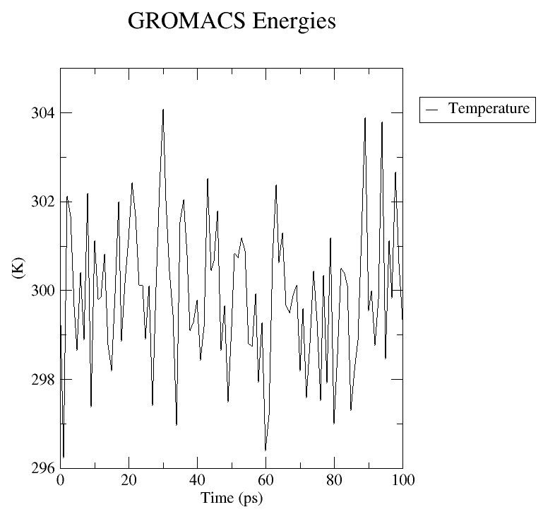
NPT平衡
构建下列npt.mdp文件,注意标黄列的名称与上述索引组名称一致:
title                   = Protein-ligand complex NPT equilibration
define                  = -DPOSRES  ; position restrain the protein and ligand
; Run parameters
integrator              = md        ; leap-frog integrator
nsteps                  = 50000     ; 2 * 50000 = 100 ps
dt                      = 0.002     ; 2 fs
; Output control
nstenergy               = 500       ; save energies every 1.0 ps
nstlog                  = 500       ; update log file every 1.0 ps
nstxout-compressed      = 500       ; save coordinates every 1.0 ps
; Bond parameters
continuation            = yes       ; continuing from NVT
constraint_algorithm    = lincs     ; holonomic constraints
constraints             = h-bonds   ; bonds to H are constrained
lincs_iter              = 1         ; accuracy of LINCS
lincs_order             = 4         ; also related to accuracy
; Neighbor searching and vdW
cutoff-scheme           = Verlet
ns_type                 = grid      ; search neighboring grid cells
nstlist                 = 20        ; largely irrelevant with Verlet
rlist                   = 1.2
vdwtype                 = cutoff
vdw-modifier            = force-switch
rvdw-switch             = 1.0
rvdw                    = 1.2       ; short-range van der Waals cutoff (in nm)
; Electrostatics
coulombtype             = PME       ; Particle Mesh Ewald for long-range electrostatics
rcoulomb                = 1.2
pme_order               = 4         ; cubic interpolation
fourierspacing          = 0.16      ; grid spacing for FFT
; Temperature coupling
tcoupl                  = V-rescale                     ; modified Berendsen thermostat
tc-grps                 = Protein_MOL Water_and_ions    ; two coupling groups - more accurate
tau_t                   = 0.1   0.1                     ; time constant, in ps
ref_t                   = 300   300                     ; reference temperature, one for each group, in K
; Pressure coupling
pcoupl                  = Berendsen                     ; pressure coupling is on for NPT
pcoupltype              = isotropic                     ; uniform scaling of box vectors
tau_p                   = 2.0                           ; time constant, in ps
ref_p                   = 1.0                           ; reference pressure, in bar
compressibility         = 4.5e-5                        ; isothermal compressibility of water, bar^-1
refcoord_scaling        = com
; Periodic boundary conditions
pbc                     = xyz       ; 3-D PBC
; Dispersion correction is not used for proteins with the C36 additive FF
DispCorr                = no
; Velocity generation
gen_vel                 = no        ; velocity generation off after NVT
执行平衡:
gmx grompp -f npt.mdp -c nvt.gro -t nvt.cpt -r nvt.gro -p topol.top -n index.ndx -o npt.tpr

gmx mdrun -deffnm npt -v最终输出的NPT状态如下:
step 50000, remaining wall clock time:     0 s
               Core t (s)   Wall t (s)        (%)
       Time:      992.000      124.000      800.0
                 (ns/day)    (hour/ns)
Performance:       69.679        0.344
显示压力平衡过程图,选择 "16 0" Pressure ,并查看:
gmx energy -f npt.edr -o pressure.xvg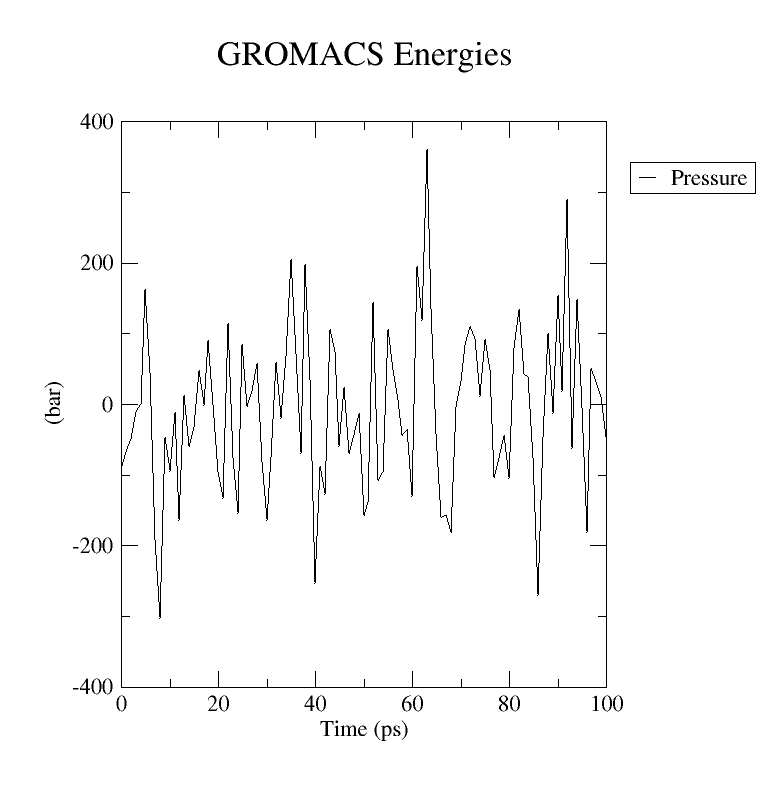
显示压力平衡过程图,选择 “22 0" Density ,并查看:
gmx energy -f npt.edr -o density.xvg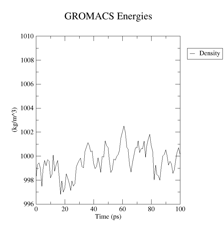
开始模拟
构建以下md.mdp文件,设置合理时间(标红列),一般是大于100ns。同时还要注意标黄列的名称与上述索引组名称一致:
title                   = Protein-ligand complex MD simulation
; Run parameters
integrator              = md        ; leap-frog integrator
nsteps                  = 5000000   ; 2 * 5000000 = 10000 ps (10 ns)
dt                      = 0.002     ; 2 fs
; Output control
nstenergy               = 5000      ; save energies every 10.0 ps
nstlog                  = 5000      ; update log file every 10.0 ps
nstxout-compressed      = 5000      ; save coordinates every 10.0 ps
; Bond parameters
continuation            = yes       ; continuing from NPT
constraint_algorithm    = lincs     ; holonomic constraints
constraints             = h-bonds   ; bonds to H are constrained
lincs_iter              = 1         ; accuracy of LINCS
lincs_order             = 4         ; also related to accuracy
; Neighbor searching and vdW
cutoff-scheme           = Verlet
ns_type                 = grid      ; search neighboring grid cells
nstlist                 = 20        ; largely irrelevant with Verlet
rlist                   = 1.2
vdwtype                 = cutoff
vdw-modifier            = force-switch
rvdw-switch             = 1.0
rvdw                    = 1.2       ; short-range van der Waals cutoff (in nm)
; Electrostatics
coulombtype             = PME       ; Particle Mesh Ewald for long-range electrostatics
rcoulomb                = 1.2
pme_order               = 4         ; cubic interpolation
fourierspacing          = 0.16      ; grid spacing for FFT
; Temperature coupling
tcoupl                  = V-rescale                     ; modified Berendsen thermostat
tc-grps                 = Protein_MOL Water_and_ions    ; two coupling groups - more accurate
tau_t                   = 0.1   0.1                     ; time constant, in ps
ref_t                   = 300   300                     ; reference temperature, one for each group, in K
; Pressure coupling
pcoupl                  = Parrinello-Rahman             ; pressure coupling is on for NPT
pcoupltype              = isotropic                     ; uniform scaling of box vectors
tau_p                   = 2.0                           ; time constant, in ps
ref_p                   = 1.0                           ; reference pressure, in bar
compressibility         = 4.5e-5                        ; isothermal compressibility of water, bar^-1
; Periodic boundary conditions
pbc                     = xyz       ; 3-D PBC
; Dispersion correction is not used for proteins with the C36 additive FF
DispCorr                = no
; Velocity generation
gen_vel                 = no        ; continuing from NPT equilibration
执行命令,启动模拟,利用GPU加速,并输出详细步骤:
gmx grompp -f md.mdp -c npt.gro -t npt.cpt -p topol.top -n index.ndx -o md_0.tpr

gmx mdrun -deffnm md_0 -nb gpu -v
结果分析
最终的运行输出如下:
step 5000000, remaining wall clock time:     0 s
               Core t (s)   Wall t (s)        (%)
       Time:   104976.000    13122.000      800.0
                         3h38:42
                 (ns/day)    (hour/ns)
Performance: 65.844 0.364若模拟计算中途中断,可使用-cpi在中断处续跑,其中md_0.cpt是中断前产生的文件:
gmx mdrun -deffnm md_0 -nb gpu -cpi md_0.cpt -v矫正轨迹
TIP
为什么要进行矫正?
- 解决周期性边界条件(PBC)问题
在MD模拟中,系统通常使用周期性边界条件(PBC),分子可能在模拟盒子边缘“断裂”(例如,一个水分子的一部分在盒子左侧,另一部分在右侧)。使用 -pbc mol 会重新包装分子,确保每个分子是完整的(基于质量中心位置)。
- 将轨迹居中(便于可视化与分析)
-center 将选定的组(默认为组 1,通常是蛋白质)置于盒子中心,避免分子在盒子边缘漂移,使轨迹更易观察(如用VMD或PyMOL可视化时)。
- 优化盒子形状
-ur compact 将系统放入最小的矩形(正交)盒子,避免模拟盒子中有空洞(例如,菱形盒子转换为紧凑的矩形盒子),提高后续分析效率。
调用 trjconv 来执行操作:
gmx trjconv -s md_0.tpr -f md_0.xtc -o md_0_center.xtc -center -pbc mol -ur compact选择 “1 Protein” 进行居中,选择 “0 System” 进行输出,得到居中后的轨迹文件 md_0_center.xtc
在后续计算中需要起始帧做参比,使用 trjconv -dump 提取轨迹的第一帧 (t = 0 ns),并选择载入的是重新居中的轨迹文件 md_0_center.xtc:
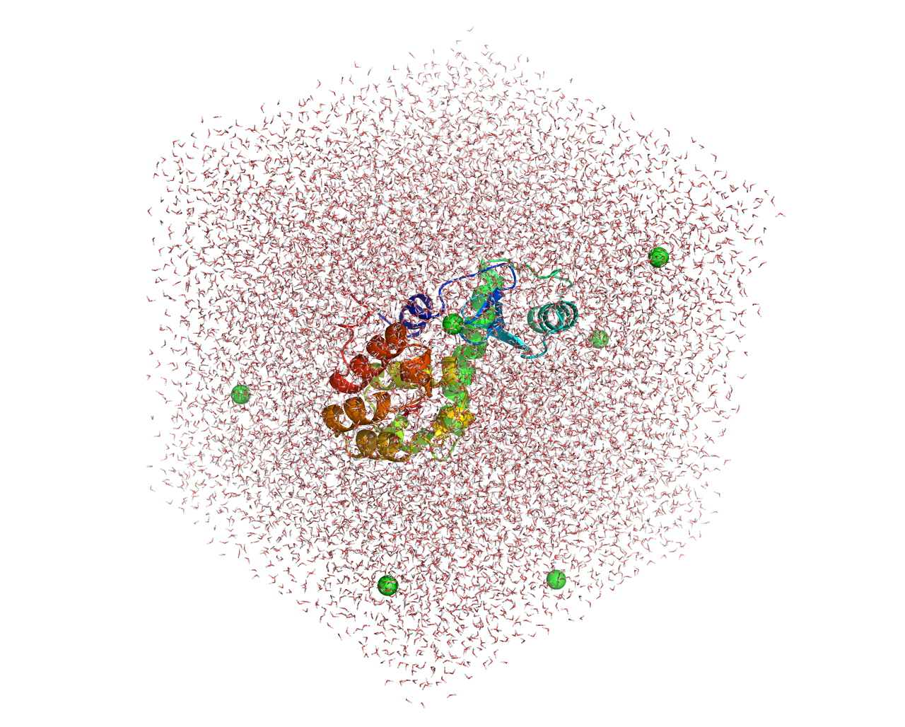
gmx trjconv -s md_0.tpr -f md_0_center.xtc -o start.pdb -dump 0选择 “0 System” 进行输出,得到居中后的起始帧文件 start.pdb,它包含所有原子(蛋白、水、离子等),适合后续全体系分析或重启模拟。
使用pymol可以可视化查看起始帧文件:
执行下列命令,获得更平滑的可视化,同时执行旋转和平移拟合,消除分子整体平动和转动,使轨迹更适合分析:
gmx trjconv -s md_0.tpr -f md_0_center.xtc -o md_0_fit.xtc -fit rot+trans选择 “4 Backbone” 对蛋白质骨架进行最小二乘拟合,选择 “0 System” 进行输出,得到拟合后的轨迹文件 md_0_fit.xtc。
利用VMD或pymol载入md_0.gro和md_0_fit.xtc轨迹文件,即可查看可视化动画:
结构稳定性分析
分子动力学(MD)模拟数据的数据分析主要包括 结构稳定性分析 和 能量分析 ,涵盖 RMSD、RMSF、Rg、氢键、SASA、自由能形貌图 以及 MMPBSA结合自由能计算 和 残基能量分解,均可使用GROMACS和辅助工具(python)完成,后文将详细介绍每部分的分析方法。
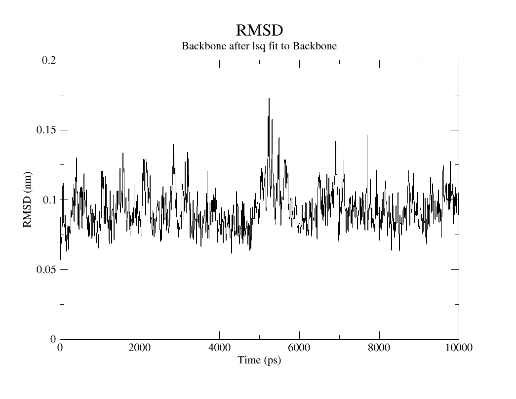
RMSD(均方根偏差)
作用:评估蛋白质整体结构的稳定性(相对于初始构象的偏差)。
命令:
gmx rms -s md_0.tpr -f md_0_fit.xtc -o rmsd.xvg- 交互选择:
- 拟合组:
Backbone(或C-alpha) - 计算组:
Backbone
- 拟合组:
- 输出:
rmsd.xvg(时间 vs. RMSD,单位:nm) - 可视化:蛋白质整体结构随时间的变化幅度
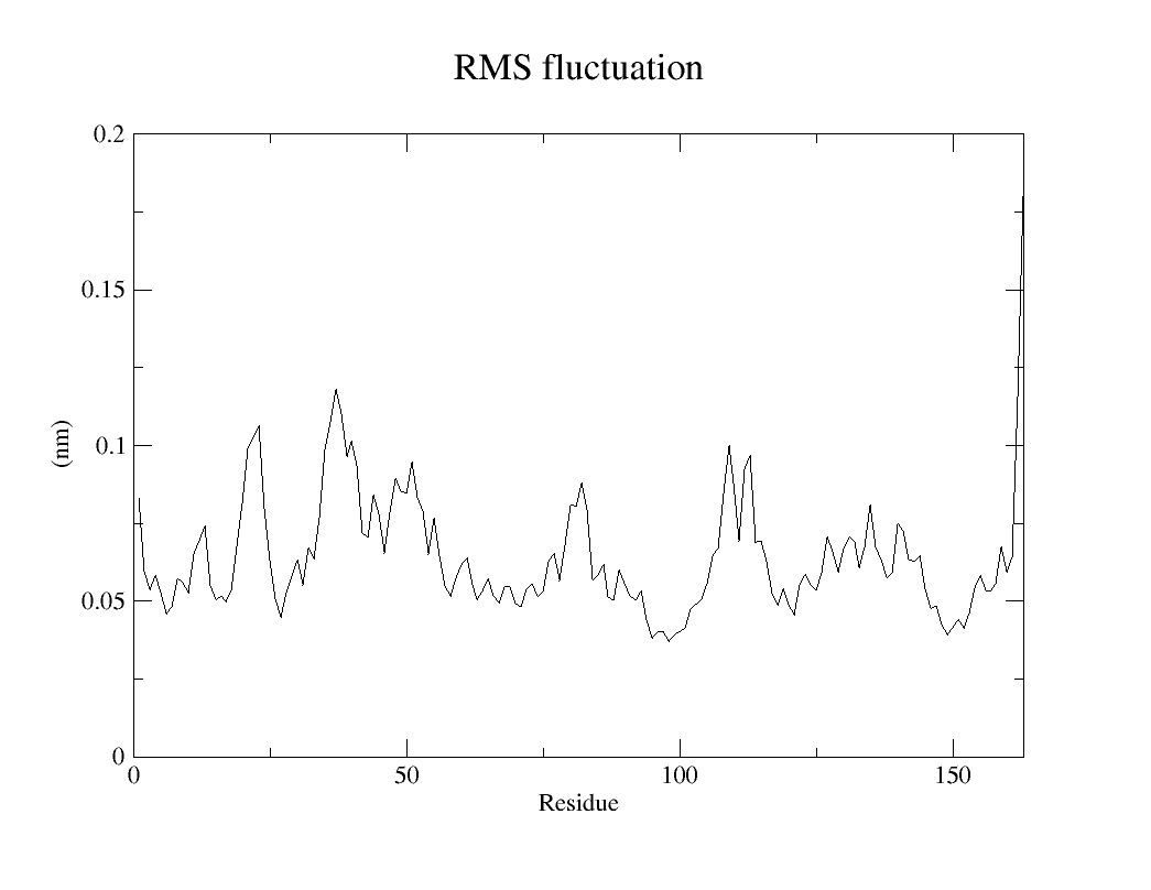
RMSF(均方根波动)
作用:分析残基的柔性(波动性),识别活性位点或柔性区域。
命令:
gmx rmsf -s md_0.tpr -f md_0_fit.xtc -o rmsf.xvg -res- 交互选择:
Backbone或Protein - 输出:
rmsf.xvg(残基编号 vs. RMSF,单位:nm) - 绘图:可以看到该蛋白质的163个氨基酸残基柔性
B因子(温度因子,B-factor)
作用:在分子动力学模拟中表征原子位置波动性的重要指标,与实验结构(如X射线晶体学或冷冻电镜)中的B因子意义一致。
命令:
gmx rmsf -s md_0.tpr -f md_0_fit.xtc -o rmsf_B.xvg -oq bfactor.pdb -res- 交互选择:选择计算组(通常为
Protein或Backbone)。 - 输出:
-oq bfactor.pdb:输出包含B因子的PDB文件,可直接用PyMOL、VMD可视化。
GROMACS的 rmsf 工具直接输出的 bfactor.pdb 已自动将RMSF(单位:nm)转换为B因子(单位:Ų):
(注:1 nm² = 100 Ų)
可视化:
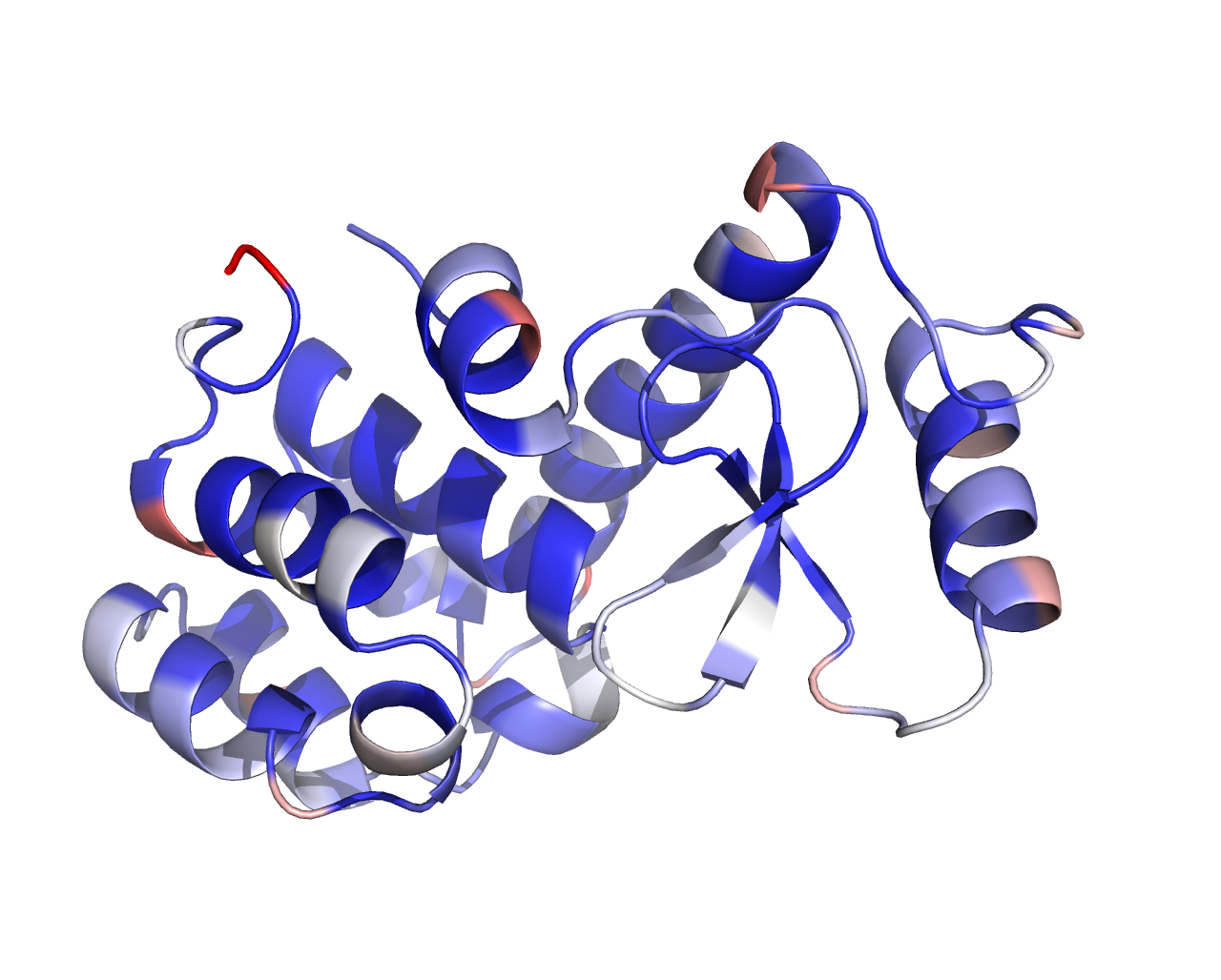
使用pymol打开bfactor.pdb文件后,输入以下命令:
spectrum b, blue_white_red, minimum=0, maximum=100得到蛋白质结构可视化图像,柔性区域(高B因子)显示为红色,刚性区域(低B因子)为蓝色:颜色的深浅变化代表了 B-factor 值的高低。
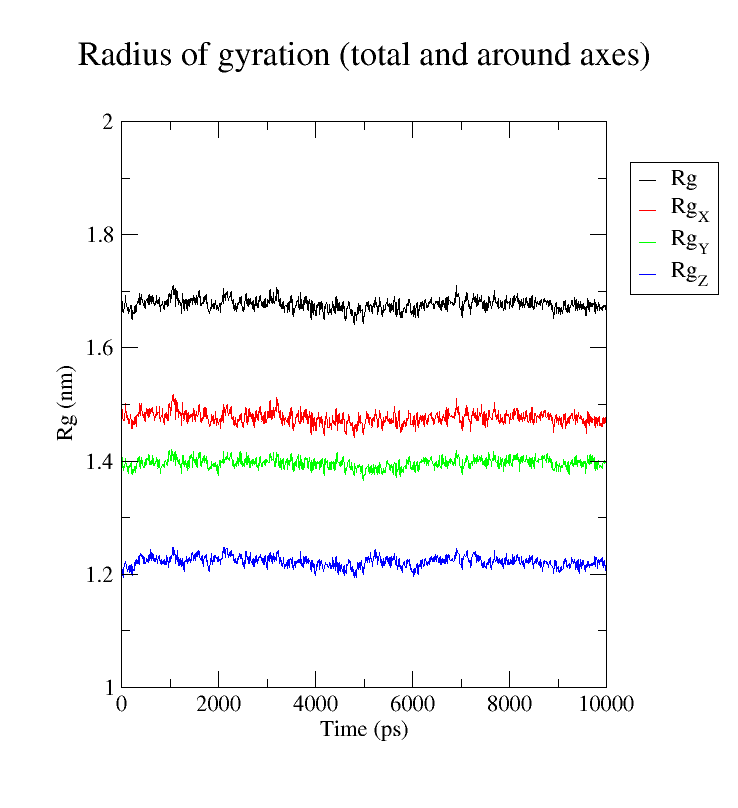
Rg(回转半径)
作用:衡量蛋白质的紧凑性(折叠/展开状态)。
命令:
gmx gyrate -s md_0.tpr -f md_0_fit.xtc -o gyrate.xvg- 交互选择:
Protein - 输出:
gyrate.xvg(时间 vs. Rg,单位:nm) - 绘图:可以看到蛋白质三个坐标方向的回转半径随时间变化曲线
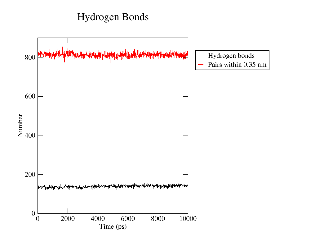
氢键(HBonds)
作用:统计氢键数量及关键残基间的氢键。
(1) 分析蛋白质内部氢键 选择供体组:1 Protein(蛋白质所有可能供体),受体组:1 Protein(蛋白质所有可能受体)
命令:
gmx hbond -s md_0.tpr -f md_0_fit.xtc -num hbnum.xvg- 输出:
hbnum.xvg:时间 vs. 氢键数量hbond.ndx:氢键对列表(可用gmx mindist进一步分析特定残基)
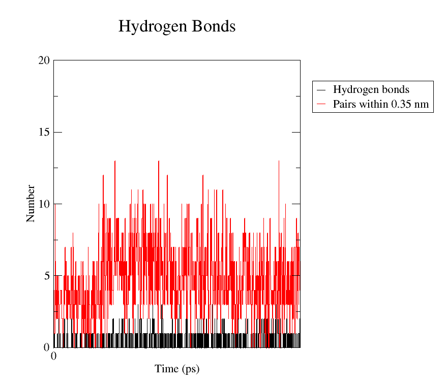
(2) 分析蛋白质-配体/水分子氢键
载入索引组,选择复合物:1 Protein(蛋白质作为氢键供体),受体组:13 MOL(小分子做氢键受体)
命令:
gmx hbond -s md_0.tpr -f md_0_fit.xtc -num hbnum_complex.xvg -n index.ndx- 输出:
hbnum_complex.xvg:时间 vs. 氢键数量hbond_complex.ndx:氢键对列表(可用gmx mindist进一步分析特定残基)
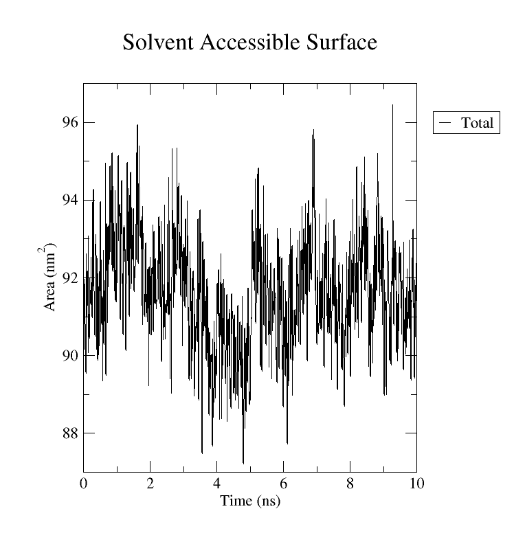
SASA(溶剂可及表面积)
作用:分析蛋白质折叠/展开状态、疏水核心暴露程度。
命令:
gmx sasa -s md_0.tpr -f md_0_fit.xtc -o sasa.xvg -tu ns- 交互选择:
1 Protein - 输出:
sasa.xvg(时间 vs. SASA,单位:nm²) - 结果分析:SASA值增大,可能表示蛋白质解折叠或局部结构松动;SASA值减小,可能反映蛋白质构象收缩或聚集。
自由能形貌图(FEL)
作用:通过降维投影(如PCA)构建自由能景观。
步骤: 在接下来的绘制中,需要先安装绘图工具,例如DuIvyTools,输入如下命令安装:
pip install DuIvyTools接下来需要处理文件,将rmsd.xvg和gyrate.xvg的数据列合并在一起,并删除x、y、z三个分量的数据,只保留时间、rmsd、Rg三列数据,保存至RMSD_Rg.xvg文件,最终文件的内容应该如下:
0 0.0005029 2.08542
10  0.08738 2.11151
20  0.10294 2.11733
30  0.12788 2.11688
40  0.13387 2.12032
50  0.12505 2.12589
60  0.12247 2.11993
70  0.12725 2.11907
80  0.14401 2.11781
90  0.14772 2.1241
100 0.15343 2.12551
110 0.15198 2.11755
120 0.15491 2.1219
130 0.13968 2.11864
140 0.14124 2.12206
150 0.14824 2.13163
160 0.15263 2.13902
170 0.14406 2.13907
180 0.15069 2.12369
190 0.14426 2.13104
200 0.14003 2.12969
210 0.1314 2.118输入下列命令,得到gibbs.xpm文件,即为自由能结果:
gmx sham -f RMSD_Rg.xvg生成2D自由能形貌图:
dit xpm_show -f gibbs.xpm -x "RMSD (nm)" -y "Rg (nm)"生成3D自由能形貌图:
dit xpm_show -f gibbs.xpm -eg plotly -m 3d -cmap spectral -x "RMSD (nm)" -y "Rg (nm)"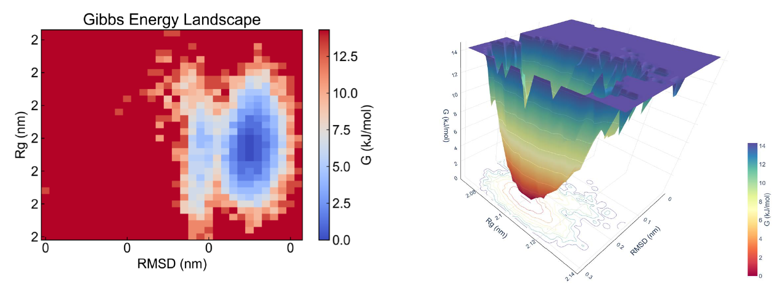
利用主成分绘制FEL
一般来说利用主成分绘制FEL,也就是用主成分1和主成分2取代上文的rmsd和gyrate,后面的处理就都是一样的。
要获得主成分,需要对轨迹进行主成分分析,gmx提供了covar命令和anaeig命令帮助我们进行相关分析。请一定注意要在PCA之前消除轨迹的平动和转动,以免分子的整体运动影响分子内部运动的分析。
covar命令的作用是对轨迹进行协方差矩阵和本征向量的计算:
gmx covar -s md_0.tpr -f md_0_fit.xtc -o eigenvalues.xvg -v eigenvectors.trr -xpma covapic.xpm按提示选择使用哪些原子做align,选3 C-alpha或者4 backbone,之后选择对哪些原子做PCA,也选C-alpha或者backbone。
eigenvalues.xvg里面记录了分析得出的多个本征值的序号和大小,对于FEL来说,我们通常希望前两个本征值的大小的和可以越大越好,这意味着前两个主成分就可以代表蛋白的大部分运动信息。
eigenvectors.trr即是投影到本征向量之后的轨迹,covapic.xpm即是轨迹的协方差矩阵。
利用anaeig命令将轨迹投影到前两个主成分上,得到pc1.xvg和pc2.xvg文件,它们在之后绘制FEL中的作用就同于前面rmsd.xvg和gyrate.xvg。
gmx anaeig -s md_0.tpr -f md_0_fit.xtc -v eigenvectors.trr -first 1 -last 1 -proj pc1.xvg

gmx anaeig -s md_0.tpr -f md_0_fit.xtc -v eigenvectors.trr -first 2 -last 2 -proj pc2.xvg之后组合两个主成分,得到pc12_sham.xvg文件,然后利用sham命令生成自由能形貌图:
gmx sham -tsham 310 -nlevels 100 -f pc12_sham.xvg -ls pc12_gibbs.xpm -g pc_12.log -lsh pc12_enthalpy.xpm -lss pc12_entropy.xpm生成的pc12_gibbs.xpm可进行可视化:
dit xpm_show -f pc12_gibbs.xpm
我们发现,通过前两个主成分做出来的FEL和通过RMSD、Gyrate做出来的FEL并不一样。是的,因为它们代表了蛋白不同尺度(或者方向)上的运动,对于蛋白的表示不同,得到的FEL也会不同。文献当中,这两种FEL的绘制方式都很常见。
能量分析
本文后续的计算分析需要借助Linux系统的AmberTools和gmx_MMPBSA来完成,请 参照本站前文的安装方法在Linux系统上正确安装软件包后进行操作。
MM-PBSA 结合自由能计算
作用:估算蛋白质-配体结合自由能(ΔGbind)。
步骤:
新建以下的mmpbsa.in文件:
&general
sys_name="Prot-Lig-CHARMM",
startframe=1,
endframe=10,
#PBRadii=7,
/
&pb
istrng=0.15,
fillratio=4.0,
radiopt=0
/
&decomp
idecomp=2,
dec_verbose=3,
print_res="within 4"
/运行下列命令,可以根据需求设置-np参数的cpu核数:
mpirun -np 8 gmx_MMPBSA -O -i mmpbsa.in -cs com.tpr -ci index.ndx -cg 1 13 -ct com_traj.xtc -cp topol.top若出现报错,请根据提示自行查证,最常见的错误是拓扑文件丢失或名称不对应,按照提示改正即可,运行成功的标志是生成了 FINAL_DECOMP_MMPBSA.dat、FINAL_RESULTS_MMPBSA.dat文件,随后将会自动打开一个图形化界面,在此界面完成数据分析即可。
残基能量分解
作用:识别对结合自由能贡献大的残基。
FINAL_RESULTS_MMPBSA.dat文件里记录了体系的各项总能量数据,包含四个统计表,表的各项释义如下:
| 能量组分 | 含义 |
|---|---|
| BOND | 键能 |
| ANGLE | 角能 |
| DIHED | 二面角能 |
| VDWAALS | 范德华力 |
| EEL | 静电势能 |
| 1 - 4 VDW | 分子中相隔3个键的原子对的范德华作用 |
| 1 - 4 EEL | 相隔3个键的原子对的静电相互作用能量 |
| EPB | 溶剂化自由能 |
| ENPOLAR | 非极性溶剂化自由能 |
| EDISPER | |
| GGAS | 分子力学项 |
| GSOLV | 分子溶剂化项 |
| TOTAL | 总能量 |
复合物各项能量组分

受体各项能量组分

配体各项能量组分

总自由能变化

将以上数据归类借助数据分析可视化软件可得到如下统计图表:

FINAL_DECOMP_MMPBSA.dat文件记录了每个氨基酸残基对体系自由能的贡献,同样借助统计可视化软件的可到如下图表:

至此,就完成了蛋白配体复合物动力学模拟及数据分析的全流程。