案例一 水中溶菌酶

这个示例将指导新用户完成设置模拟系统的过程，该系统在一盒水中含有蛋白质 （溶菌酶） 和离子。每个步骤都将包含输入和输出的说明，使用一般使用的典型设置。

整个教程的步骤如下：

准备拓扑文件

PDB检索

在模拟开始前下载大分子pdb文件，通常是在RCSB数据库官网下载，在本教程中，我们将使用鸡蛋清溶菌酶（PDB 代码1AKI）

下载结构后，使用 VMD、Chimera、PyMOL 等查看程序可视化结构。

去水

接下来要处理大分子文件，删除水分子（PDB 文件中的 HOH），请使用 vim（Linux/Mac） 或记事本 （Windows） 等纯文本编辑器，这里推荐统一使用VScode，配置工作路径和gmx插件后使用。

使用Pymol等软件去水同样可以。

并不是每次都要去水（例如有紧密结合或其他功能性活性位点水分子的情况），本案例中不需要水分子。

生成拓扑

完成水分子去除后，PDB文件应该只包含蛋白质原子，使用 pdb2gmx 模块构建拓扑（默认为 topol.top），文件中记载了仿真中定义分子所需的所有信息。此信息包括非键合参数（原子类型和电荷）以及键合参数（键、角度和二面体）。

使用以下命令选择力场，构建蛋白质拓扑：

gmx pdb2gmx -f 1AKI_clean.pdb -o 1AKI_processed.gro -water spce

在本教程中我们将使用全原子OPLS力场，因此在命令提示符下键入15：

Select the Force Field:
From '/usr/local/gromacs/share/gromacs/top':
 1: AMBER03 protein, nucleic AMBER94 (Duan et al., J. Comp. Chem. 24, 1999-2012, 2003)
 2: AMBER94 force field (Cornell et al., JACS 117, 5179-5197, 1995)
 3: AMBER96 protein, nucleic AMBER94 (Kollman et al., Acc. Chem. Res. 29, 461-469, 1996)
 4: AMBER99 protein, nucleic AMBER94 (Wang et al., J. Comp. Chem. 21, 1049-1074, 2000)
 5: AMBER99SB protein, nucleic AMBER94 (Hornak et al., Proteins 65, 712-725, 2006)
 6: AMBER99SB-ILDN protein, nucleic AMBER94 (Lindorff-Larsen et al., Proteins 78, 1950-58, 2010)
 7: AMBERGS force field (Garcia & Sanbonmatsu, PNAS 99, 2782-2787, 2002)
 8: CHARMM27 all-atom force field (CHARM22 plus CMAP for proteins)
 9: GROMOS96 43a1 force field
10: GROMOS96 43a2 force field (improved alkane dihedrals)
11: GROMOS96 45a3 force field (Schuler JCC 2001 22 1205)
12: GROMOS96 53a5 force field (JCC 2004 vol 25 pag 1656)
13: GROMOS96 53a6 force field (JCC 2004 vol 25 pag 1656)
14: GROMOS96 54a7 force field (Eur. Biophys. J. (2011), 40,, 843-856, DOI: 10.1007/s00249-011-0700-9)
15: OPLS-AA/L all-atom force field (2001 aminoacid dihedrals)。

pdb2gmx的常见参数如下：

-ignh：忽略 PDB 文件中的 H 原子;特别适用于核磁共振结构。否则，如果存在 H 原子，则它们必须按照 GROMACS 中的力场期望的命名方式命名。

-ter：交互式地为 N 端和 C 端分配电荷态。

-inter：交互式地为 Glu、Asp、Lys、Arg 和 His 分配电荷态；选择哪些 Cys 参与二硫键。

程序运行完成后会生成如下三个文件，1AKI_processed.gro 是一个 GROMACS 格式的结构文件，其中包含力场中定义的所有原子（完成加氢），topol.top 文件是系统拓扑，posre.itp 文件包含用于约束重原子位置的信息。

dir/
├── posre.itp                 # 蛋白的位置限制文件
├── 1AKI_processed.gro        # 蛋白gro文件
└── topol.top                 # 体系拓扑文件

GROMACS 可以处理许多不同的文件格式，.gro 只是写入坐标文件命令的默认值，也可以指定程序输出 .pdb 文件。

检查拓扑

topol.top

输出拓扑 topol.top 文件，可以使用纯文本编辑器打开。;符号表示为注释行。

#include "oplsaa.ff/forcefield.itp"

此行调用 OPLS-AA 力场中的参数，它位于文件的开头，表示所有后续参数都来自此力场。

下一个重要行是[ moleculetype ]：

[ moleculetype ]

; Name       nrexcl
Protein_A    3

名称 Protein_A 定义了分子名称，因为蛋白质在 PDB 文件中被标记为链 A 的事实。绑定邻域有 3 个排除项。

下一节[ atoms ]定义了蛋白中的氨基酸序列，信息以列的形式显示：

[ atoms ]
;   nr       type  resnr residue  atom   cgnr     charge       mass  typeB    chargeB      massB
; residue   1 LYS rtp LYSH q +2.0
     1   opls_287      1   LYS       N      1       -0.3    14.0067   ; qtot -0.3
     2   opls_290      1   LYS      H1      1       0.33      1.008   ; qtot 0.03
     3   opls_290      1   LYS      H2      1       0.33      1.008   ; qtot 0.36
     4   opls_290      1   LYS      H3      1       0.33      1.008   ; qtot 0.69
     5  opls_293B      1   LYS      CA      1       0.25     12.011   ; qtot 0.94
     6   opls_140      1   LYS      HA      1       0.06      1.008   ; qtot 1

本节信息解读如下：

• nr：原子数
• type： 原子型
• resnr：氨基酸残基数
• residue：氨基酸残基名称；请注意，此残基在 PDB 文件中为 “LYS”;使用 .rtp ，“LYSH”表示残基是质子化的（中性 pH 值下的主要状态）。
• atom： 原子名称
• cgnr：电荷组编号；电荷组定义整数电荷的单位，它们有助于加快计算速度
• charge： qtot 描述符是分子上电荷的运行总和
• mass：质量
• typeB， chargeB， massB： 用于自由能扰动（此处不讨论）

[ bonds ]是化学键, [ pairs ]原子非键合作用力, [ angles ]表示二键角, [ dihedrals ]表示二面角。

Protein_A 分子型定义到此结束，拓扑文件的其余部分专门用于定义其他分子并提供系统级描述，主要包括位置约束等。

; Include Position restraint file
#ifdef POSRES
#include "posre.itp"
#endif

下一个分子型（默认）是溶剂，在本例中为 SPC/E 水。其他典型的水选择包括 SPC、TIP3P 和 TIP4P。我们通过将 -water spce 传递给 pdb2gmx 来选择它。

水也可以使用 1000 kJ mol-1 nm-2 的力常数 （kpr） 进行位置约束。

; Include water topology
#include "oplsaa.ff/spce.itp"

#ifdef POSRES_WATER
; Position restraint for each water oxygen
[ position_restraints ]
;  i funct       fcx        fcy        fcz
   1    1       1000       1000       1000
#endif

接下来包括离子参数：

; Include generic topology for ions
#include "oplsaa.ff/ions.itp"

最后是系统级定义，该指令给出了在仿真期间将写入输出文件的系统的名称，该指令列出了系统中的所有分子：

[ system ]
; Name
LYSOZYME

[ molecules ]
; Compound        #mols
Protein_A           1

关于该指令的一些关键说明：

• 列出的分子的顺序必须与坐标（在本例中为 .gro）文件中的分子顺序完全匹配。
• 列出的名称必须与每个物种的名称相匹配，而不是残留物名称或其他任何内容。
• 如果这些具体要求没有符合条件， grompp 将会抛出致命错误，例如名称不匹配、未找到分子或许多其他错误。

posre.itp

posre.itp 是位置限制文件，由 pdb2gmx 生成，它定义了一个力常数，用于在平衡过程中将原子保持在原位。

示例：

[ position_restraints ]
; atom  type      fx      fy      fz
     1     1  1000  1000  1000
     5     1  1000  1000  1000
     7     1  1000  1000  1000
    10     1  1000  1000  1000
    13     1  1000  1000  1000

溶剂化

本案例中我们将模拟一个简单的水性系统，动力学模拟时需要设置合适的盒子大小，整个系统的计算将在该范围内完成。

设置盒子

本例使用一个简单的立方框作为基本单元，它的体积计算最为简单，此外还可以选择菱形十二面体盒子，它的体积是相同周期距离的立方框的71%，空间利用度高，从而节提升了计算效率。

定义盒子并在其中填充溶剂有两个步骤：

1. 使用editconf模块定义盒子尺寸
2. 使用 solvate模块将盒子装满水。

输入如下命令生成盒子：

gmx editconf -f 1AKI_processed.gro -o 1AKI_newbox.gro -c -d 1.0 -bt cubic

上述命令将蛋白质在框 （-c） 中居中，并将其放置在距框边缘至少 1.0 nm （-d 1.0） 的位置。框类型定义为多维数据集 （-bt cubic）。到框边缘的距离是一个重要参数。由于我们将使用周期性边界条件，因此必须满足最小图像约定。也就是说，蛋白质永远不应该看到它的周期性图像，否则计算的力将是虚假的。指定 1.0 nm 的溶质盒距离意味着蛋白质的任意两个周期性图像之间至少有 2.0 nm。这个距离对于模拟中常用的几乎任何截止方案都足够了。

溶剂化

使用如下命令为刚刚生成的盒子中添加溶剂分子：

gmx solvate -cp 1AKI_newbox.gro -cs spc216.gro -o 1AKI_solv.gro -p topol.top

我们使用的是spc216.gro，这是一个通用的平衡 3 点溶剂模型。您可以使用spc216.gro作为 SPC、SPC/E 或 TIP3P 水的溶剂配置，因为它们都是三点水模型。程序会得到一个名为1AKI_solv.gro的文件。

观察到 topol.top 文件的末尾会出现如下行，这是gmx程序成功添加了10832个水分子，如果使用的是其他溶剂，则需要手动修改该文件：

[ molecules ]
; Compound  #mols
Protein_A       1 
SOL         10832

添加离子

我们现在有一个包含带电蛋白质的溶剂化系统。上文中的 pdb2gmx 输出提示我们，该蛋白质的净电荷为 +8e（基于其氨基酸组成），由于生命不以净电荷存在，因此我们必须将离子添加到我们的系统中。

构建下列ions.mdp文件：

; ions.mdp - used as input into grompp to generate ions.tpr
; Parameters describing what to do, when to stop and what to save
integrator  = steep         ; Algorithm (steep = steepest descent minimization)
emtol       = 1000.0        ; Stop minimization when the maximum force < 1000.0 kJ/mol/nm
emstep      = 0.01          ; Minimization step size
nsteps      = 50000         ; Maximum number of (minimization) steps to perform

; Parameters describing how to find the neighbors of each atom and how to calculate the interactions
nstlist         = 1         ; Frequency to update the neighbor list and long range forces
cutoff-scheme	= Verlet    ; Buffered neighbor searching 
ns_type         = grid      ; Method to determine neighbor list (simple, grid)
coulombtype     = cutoff    ; Treatment of long range electrostatic interactions
rcoulomb        = 1.0       ; Short-range electrostatic cut-off
rvdw            = 1.0       ; Short-range Van der Waals cut-off
pbc             = xyz       ; Periodic Boundary Conditions in all 3 dimensions

输入以下命令使用grompp生成tpr文件：

gmx grompp -f ions.mdp -c 1AKI_solv.gro -p topol.top -o ions.tpr

最后使用genion模块为体系加离子，使得整个体系变为电中性：

gmx genion -s ions.tpr -o 1AKI_solv_ions.gro -p topol.top -pname NA -nname CL -neutral

程序会提示选择哪个分组来添加离子，选择索引组 SOL (13) 进行嵌入离子，合理的情况应该是替换溶剂分子，而不是选择蛋白或小分子，因为这样会破坏其分子结构：

此时的topol.top文件的[ molecules ]块末尾应增加如下行：

[ molecules ]
; Compound      #mols
Protein_A         1
SOL           10636
CL                8

此时的1AKI_solv_ions.gro文件如下：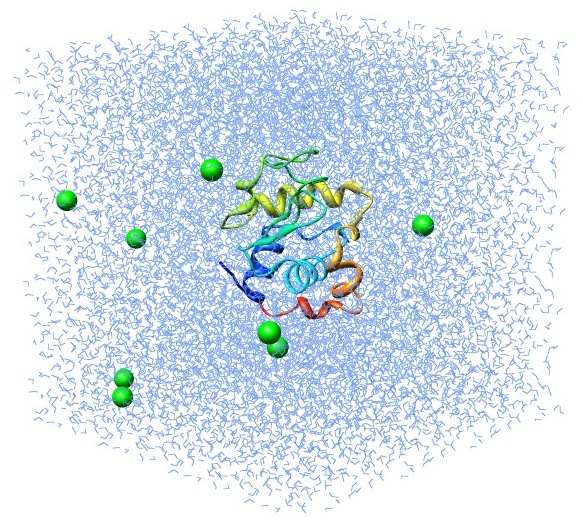

能量最小化

溶剂化的电中性系统现已组装完成，在开始动力学之前，我们必须确保系统没有空间冲突或不适当的几何图形。该结构通过称为能量最小化的过程而松弛。

EM 的过程很像离子的添加。我们将再次使用 grompp 将结构、拓扑和仿真参数组装成二进制输入文件 （.tpr），但这一次，我们将通过 GROMACS MD 引擎 mdrun 运行能量最小化，而不是将 .tpr 传递给 genion。

构建mdp文件

新建以下内容的minim.mdp文件：

; minim.mdp - used as input into grompp to generate em.tpr
; Parameters describing what to do, when to stop and what to save
integrator  = steep         ; Algorithm (steep = steepest descent minimization)
emtol       = 1000.0        ; Stop minimization when the maximum force < 1000.0 kJ/mol/nm
emstep      = 0.01          ; Minimization step size
nsteps      = 50000         ; Maximum number of (minimization) steps to perform

; Parameters describing how to find the neighbors of each atom and how to calculate the interactions
nstlist         = 1         ; Frequency to update the neighbor list and long range forces
cutoff-scheme   = Verlet    ; Buffered neighbor searching
ns_type         = grid      ; Method to determine neighbor list (simple, grid)
coulombtype     = PME       ; Treatment of long range electrostatic interactions
rcoulomb        = 1.0       ; Short-range electrostatic cut-off
rvdw            = 1.0       ; Short-range Van der Waals cut-off
pbc             = xyz       ; Periodic Boundary Conditions in all 3 dimensions

使用以下输入参数文件通过 grompp 组装二进制输入：

gmx grompp -f minim.mdp -c 1AKI_solv_ions.gro -p topol.top -o em.tpr

调用 mdrun 来执行能量最小化：

gmx mdrun -v -deffnm em

-v 参数可以输出 mdrun 的每一步的进度，-deffnm 为将定义输入和输出的文件名。运行完成后会得到以下文件：

dir/
├── em.log       # 能量最小化进程ASCII文本日志文件
├── em.edr       # 二进制能量数据文件
├── em.trr       # 二进制全精度轨迹文件
└── em.gro       # 能量最小化完成后结构文件

检验结果

要确定 EM 是否成功，需要评估两个非常重要的因素。第一个是势能（在 EM 过程结束时打印，即使没有 -v）。Epot 应为负数，并且（对于水中的简单蛋白质）约为 10 5-106，具体取决于系统大小和水分子的数量。第二个重要特征是最大力 Fmax，其目标在 minim.mdp 中设置 - “emtol = 1000.0” - 表示目标 Fmax 不大于 1000 kJ mol-1 nm-1。有可能得出一个合理的 E锅，其中 Fmax > emtol。如果发生这种情况，您的系统可能不够稳定，无法进行仿真。评估它可能发生的原因，并可能更改您的最小化参数（积分器、emstep 等）。

我们来做一些分析。em.edr 文件包含 GROMACS 在 EM 期间收集的所有能量项。您可以使用 GROMACS 能量模块分析任何 .edr 文件：

gmx energy -f em.edr -o potential.xvg

在提示符下，键入 “10 0” 以选择 Potential （10）；0 终止输入。您将看到 Epot 的平均值，并且将写入一个名为 potential.xvg 的文件。要绘制此数据，需要 Xmgrace 绘图工具。生成的图应该看起来像这样，展示了 Epot 的良好、稳定的收敛：

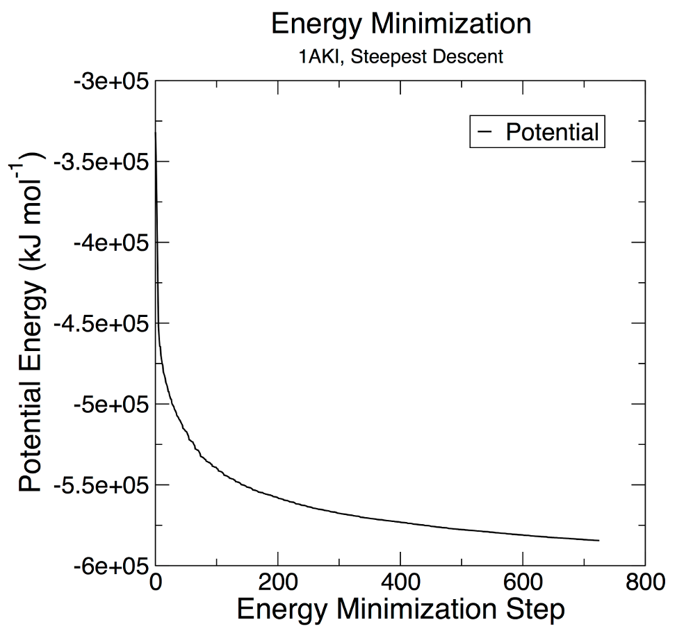
现在我们的系统处于能量最低水平，随后开始动力学模拟部分。

平衡

EM 确保我们在几何形状和溶剂取向方面具有合理的起始结构。要开始真正的动力学，我们必须平衡蛋白质周围的溶剂和离子。如果我们在这一点上尝试无拘无束的动态，系统可能会崩溃。原因是溶剂大部分内部都是优化的，而不一定是溶质的优化。需要将其加热到我们希望模拟的温度，并建立有关溶质（蛋白质）的正确方向。在我们达到正确的温度（基于动能）后，我们将对系统施加压力，直到它达到适当的密度。

上文 pdb2gmx 生成的 posre.itp 文件的目的是对蛋白质的重原子施加位置应变力，允许其移动，但需要克服大量的能量损失。这样一来，我们可以平衡蛋白质周围的溶剂，而不会轻易改变蛋白质结构，相当于固定了某些部分。

平衡通常分两个阶段进行。第一阶段在 NVT 系综（恒定的粒子数、体积和温度）下进行。在 NVT 后，系统的温度应该达到所需值左右，如果温度尚未稳定，则需要增加平衡的时间。通常NVT平衡需要50-100 ps 左右，本例将设置 100 ps 的 NVT 平衡。

温度平衡 NVT

构建下列nvt.mdp文件：

title                   = OPLS Lysozyme NVT equilibration 
define                  = -DPOSRES  ; position restrain the protein
; Run parameters
integrator              = md        ; leap-frog integrator
nsteps                  = 50000     ; 2 * 50000 = 100 ps
dt                      = 0.002     ; 2 fs
; Output control
nstxout                 = 500       ; save coordinates every 1.0 ps
nstvout                 = 500       ; save velocities every 1.0 ps
nstenergy               = 500       ; save energies every 1.0 ps
nstlog                  = 500       ; update log file every 1.0 ps
; Bond parameters
continuation            = no        ; first dynamics run
constraint_algorithm    = lincs     ; holonomic constraints 
constraints             = h-bonds   ; bonds involving H are constrained
lincs_iter              = 1         ; accuracy of LINCS
lincs_order             = 4         ; also related to accuracy
; Nonbonded settings 
cutoff-scheme           = Verlet    ; Buffered neighbor searching
ns_type                 = grid      ; search neighboring grid cells
nstlist                 = 10        ; 20 fs, largely irrelevant with Verlet
rcoulomb                = 1.0       ; short-range electrostatic cutoff (in nm)
rvdw                    = 1.0       ; short-range van der Waals cutoff (in nm)
DispCorr                = EnerPres  ; account for cut-off vdW scheme
; Electrostatics
coulombtype             = PME       ; Particle Mesh Ewald for long-range electrostatics
pme_order               = 4         ; cubic interpolation
fourierspacing          = 0.16      ; grid spacing for FFT
; Temperature coupling is on
tcoupl                  = V-rescale             ; modified Berendsen thermostat
tc-grps                 = Protein Non-Protein   ; two coupling groups - more accurate
tau_t                   = 0.1     0.1           ; time constant, in ps
ref_t                   = 300     300           ; reference temperature, one for each group, in K
; Pressure coupling is off
pcoupl                  = no        ; no pressure coupling in NVT
; Periodic boundary conditions
pbc                     = xyz       ; 3-D PBC
; Velocity generation
gen_vel                 = yes       ; assign velocities from Maxwell distribution
gen_temp                = 300       ; temperature for Maxwell distribution
gen_seed                = -1        ; generate a random seed

.mdp 文件中的几个主要的参数：

• gen_vel = yes：启动速度生成。使用不同的随机种子 （gen_seed） 会得到不同的初始速度，因此可以从相同的起始结构进行多个（不同的）仿真。
• tcoupl = V-rescale：速度重新定标恒温器是对 Berendsen 弱耦合方法的改进，该方法没有再现正确的动力学系综。 pcoupl = no：不应用压力耦合。

生成nvt.tpr文件：

gmx grompp -f nvt.mdp -c em.gro -r em.gro -p topol.top -o nvt.tpr

开始NVT平衡：

gmx mdrun -deffnm nvt

使用下列命令绘图，在提示符下键入 "16 0" Temperature ，生成体系时间-温度的曲线，如下所示：

gmx energy -f nvt.edr -o temperature.xvg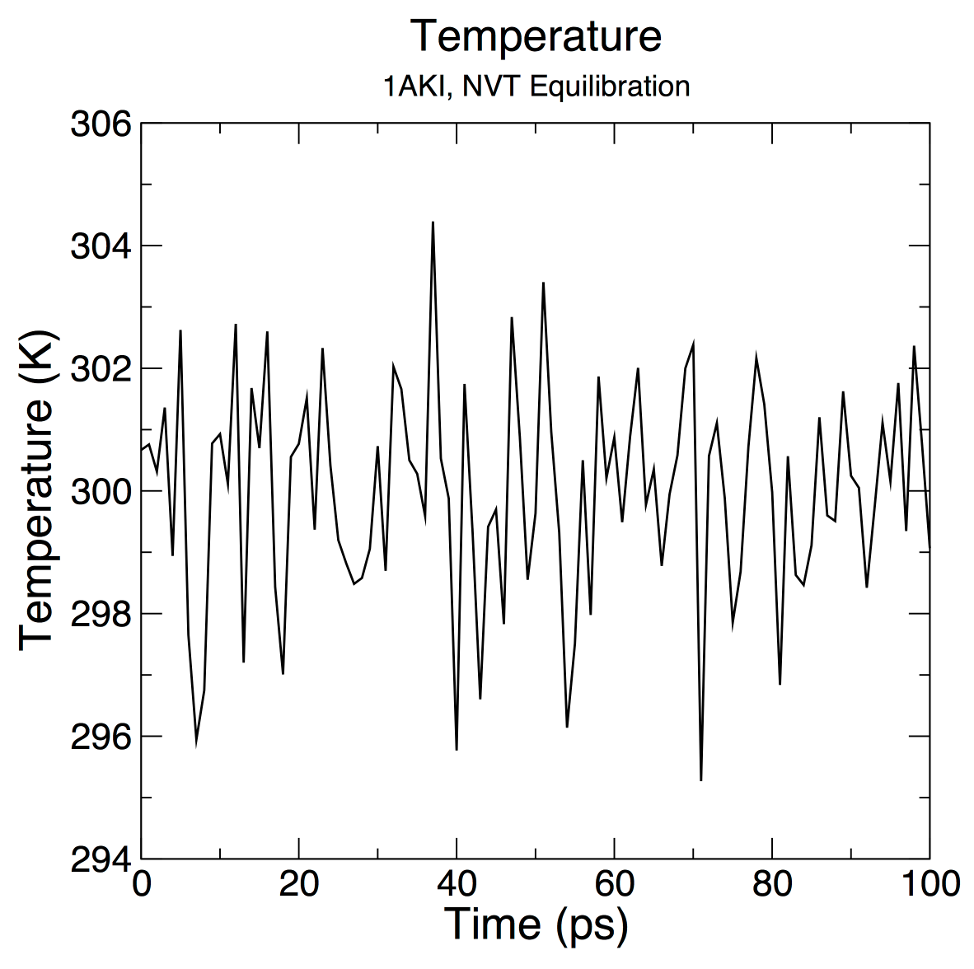

从图中可以清楚地看出，系统的温度很快达到目标值 （300 K），并且在平衡的剩余时间内保持稳定。对于该系统，较短的平衡期（大约 50 ps）可能就足够了。

压力平衡 NPT

上一步 NVT 平衡稳定了系统的温度，下一步开始稳定系统的压力（以及密度）。压力平衡在 NPT 系综下进行，其中粒子数、压力和温度都是恒定的。

构建下列 .mdp 文件：

title                   = OPLS Lysozyme NPT equilibration 
define                  = -DPOSRES  ; position restrain the protein
; Run parameters
integrator              = md        ; leap-frog integrator
nsteps                  = 50000     ; 2 * 50000 = 100 ps
dt                      = 0.002     ; 2 fs
; Output control
nstxout                 = 500       ; save coordinates every 1.0 ps
nstvout                 = 500       ; save velocities every 1.0 ps
nstenergy               = 500       ; save energies every 1.0 ps
nstlog                  = 500       ; update log file every 1.0 ps
; Bond parameters
continuation            = yes       ; Restarting after NVT 
constraint_algorithm    = lincs     ; holonomic constraints 
constraints             = h-bonds   ; bonds involving H are constrained
lincs_iter              = 1         ; accuracy of LINCS
lincs_order             = 4         ; also related to accuracy
; Nonbonded settings 
cutoff-scheme           = Verlet    ; Buffered neighbor searching
ns_type                 = grid      ; search neighboring grid cells
nstlist                 = 10        ; 20 fs, largely irrelevant with Verlet scheme
rcoulomb                = 1.0       ; short-range electrostatic cutoff (in nm)
rvdw                    = 1.0       ; short-range van der Waals cutoff (in nm)
DispCorr                = EnerPres  ; account for cut-off vdW scheme
; Electrostatics
coulombtype             = PME       ; Particle Mesh Ewald for long-range electrostatics
pme_order               = 4         ; cubic interpolation
fourierspacing          = 0.16      ; grid spacing for FFT
; Temperature coupling is on
tcoupl                  = V-rescale             ; modified Berendsen thermostat
tc-grps                 = Protein Non-Protein   ; two coupling groups - more accurate
tau_t                   = 0.1     0.1           ; time constant, in ps
ref_t                   = 300     300           ; reference temperature, one for each group, in K
; Pressure coupling is on
pcoupl                  = Parrinello-Rahman     ; Pressure coupling on in NPT
pcoupltype              = isotropic             ; uniform scaling of box vectors
tau_p                   = 2.0                   ; time constant, in ps
ref_p                   = 1.0                   ; reference pressure, in bar
compressibility         = 4.5e-5                ; isothermal compressibility of water, bar^-1
refcoord_scaling        = com
; Periodic boundary conditions
pbc                     = xyz       ; 3-D PBC
; Velocity generation
gen_vel                 = no        ; Velocity generation is off

它和之前的 NVT 平衡参数文件没有太大区别，使用 Parrinello-Rahman 恒压器添加了压力耦合部分，其他的更改如下：

• continuation = yes：我们从 NVT 平衡阶段继续模拟
• gen_vel = no：从轨迹中读取速度（见下文）

随后继续调用 grompp 和 mdrun，和NVT相同。请注意，我们现在包括 -t 标志以包含 NVT 平衡的检查点文件;此文件包含继续模拟所需的所有状态变量。为了守恒 NVT 期间产生的速度，我们必须包含此文件。坐标文件 （-c） 是 NVT 仿真的最终输出。

gmx grompp -f npt.mdp -c nvt.gro -r nvt.gro -t nvt.cpt -p topol.top -o npt.tpr

开始NPT模拟：

gmx mdrun -deffnm npt

分析结果

先使用energy来分析压力级数：

gmx energy -f npt.edr -o pressure.xvg

在提示符处键入 “18 0” 以选择系统的压力并退出。生成的绘图应如下所示：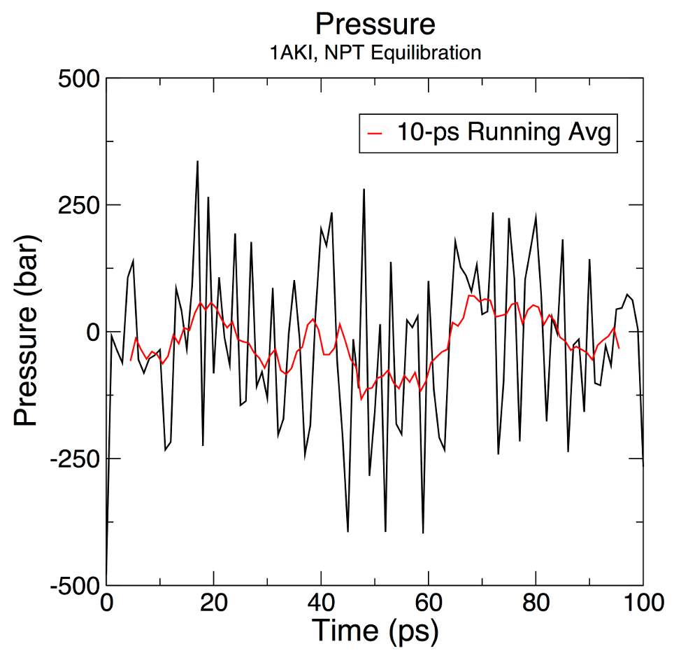

压力值在 100 ps 平衡阶段波动很大，但这种行为并不意外。这些数据的运行平均值在图中绘制为红线。在平衡过程中，压力的平均值为 7.5 ± 160.5 bar。请注意，参考压力设置为 1 bar，那么这个结果是否可以接受？压力是在 MD 模拟过程中波动很大的量，从较大的均方根波动 （160.5 bar） 中可以清楚地看出，因此从统计学上讲，无法区分获得的平均值（7.5 ± 160.5 bar）和目标/参考值（1 bar）之间的差异。

再分析密度，这次使用energy并在提示符处输入 “24 0”。

gmx energy -f npt.edr -o density.xvg

与压力一样，密度的运行平均值也用红色绘制。100 ps 过程中的平均值为 1019 ± 3 kg m-3，接近 1000 kg m-3 的实验值和 SPC/E 模型的预期密度 1008 kg m-3。SPC/E 水模型的参数与水的实验值非常相似。密度值随着时间的推移非常稳定，表明系统现在在压力和密度方面得到了很好的平衡。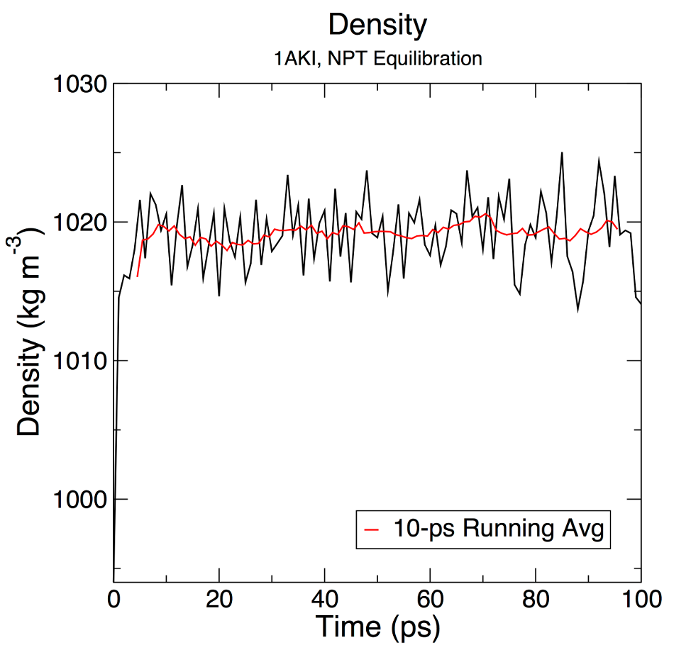

如果获得的密度值与该结果不匹配，可能是因为与压力相关的项收敛速度较慢，因此可能需要运行 NPT 平衡的时间略长于此处指定的时间。

开始模拟

完成两个平衡阶段后，系统现在在所需的温度和压力下得到很好的平衡，随后可以开始最终模拟，本例将运行 1 ns 的 MD 仿真。

构建下列的md.mdp配置文件：

title                   = OPLS Lysozyme NPT equilibration 
; Run parameters
integrator              = md        ; leap-frog integrator
nsteps                  = 500000    ; 2 * 500000 = 1000 ps (1 ns)
dt                      = 0.002     ; 2 fs
; Output control
nstxout                 = 0         ; suppress bulky .trr file by specifying 
nstvout                 = 0         ; 0 for output frequency of nstxout,
nstfout                 = 0         ; nstvout, and nstfout
nstenergy               = 5000      ; save energies every 10.0 ps
nstlog                  = 5000      ; update log file every 10.0 ps
nstxout-compressed      = 5000      ; save compressed coordinates every 10.0 ps
compressed-x-grps       = System    ; save the whole system
; Bond parameters
continuation            = yes       ; Restarting after NPT 
constraint_algorithm    = lincs     ; holonomic constraints 
constraints             = h-bonds   ; bonds involving H are constrained
lincs_iter              = 1         ; accuracy of LINCS
lincs_order             = 4         ; also related to accuracy
; Neighborsearching
cutoff-scheme           = Verlet    ; Buffered neighbor searching
ns_type                 = grid      ; search neighboring grid cells
nstlist                 = 10        ; 20 fs, largely irrelevant with Verlet scheme
rcoulomb                = 1.0       ; short-range electrostatic cutoff (in nm)
rvdw                    = 1.0       ; short-range van der Waals cutoff (in nm)
; Electrostatics
coulombtype             = PME       ; Particle Mesh Ewald for long-range electrostatics
pme_order               = 4         ; cubic interpolation
fourierspacing          = 0.16      ; grid spacing for FFT
; Temperature coupling is on
tcoupl                  = V-rescale             ; modified Berendsen thermostat
tc-grps                 = Protein Non-Protein   ; two coupling groups - more accurate
tau_t                   = 0.1     0.1           ; time constant, in ps
ref_t                   = 300     300           ; reference temperature, one for each group, in K
; Pressure coupling is on
pcoupl                  = Parrinello-Rahman     ; Pressure coupling on in NPT
pcoupltype              = isotropic             ; uniform scaling of box vectors
tau_p                   = 2.0                   ; time constant, in ps
ref_p                   = 1.0                   ; reference pressure, in bar
compressibility         = 4.5e-5                ; isothermal compressibility of water, bar^-1
; Periodic boundary conditions
pbc                     = xyz       ; 3-D PBC
; Dispersion correction
DispCorr                = EnerPres  ; account for cut-off vdW scheme
; Velocity generation
gen_vel                 = no        ; Velocity generation is off

执行MD模拟

下列命令可以将模拟参数、初始结构、拓扑信息和检查点文件整合成一个二进制文件（.tpr 文件），供后续的分子动力学模拟使用：

gmx grompp -f md.mdp -c npt.gro -t npt.cpt -p topol.top -o md_0_1.tpr

执行 mdrun开始模拟，使用-v命令会显示每一步的具体进度：

gmx mdrun -deffnm md_0_1 -v

在 GROMACS 2018 后可以调用GPU加速，只需要使用 -nb gpu 参数即可：

gmx mdrun -deffnm md_0_1 -nb gpu -V

若模拟计算中途中断，可使用-cpi在中断处续跑，其中md_0.cpt是中断前产生的文件：

gmx mdrun -deffnm md_0_1 -nb gpu -v -cpi md_0_1.cpt 12000

结果分析

现在我们已经模拟了蛋白质，我们应该对系统进行一些分析。在本教程中，将介绍一些基本动力学模拟的数据分析工具。

trjconv校正

trjconv 用作后处理工具，用于去除坐标、校正周期性或手动更改轨迹（时间单位、帧频率等）。我们使用 trjconv 来考虑系统中的任何周期性，蛋白质将通过晶胞扩散，并且可能看起来“破碎”或可能“跳”到盒子的另一侧。要考虑此类行为，请发出以下内容：

gmx trjconv -s md_0_1.tpr -f md_0_1.xtc -o md_0_1_noPBC.xtc -pbc mol -center

选择 1 （“Protein”） 作为要居中的组，选择 0 （“System”） 作为输出。我们将根据这个 “修正” 的轨迹进行所有分析。让我们先看看结构稳定性。

RMSD

GROMACS 有一个用于 RMSD 计算的内置实用程序，称为 rms，使用以下命令：

gmx rms -s md_0_1.tpr -f md_0_1_noPBC.xtc -o rmsd.xvg -tu ns

选择 4（“Backbone”）作为最小二乘拟合和 RMSD 计算的组。-tu 标志将以 ns 为单位输出结果，即使轨迹以 ps 为单位编写。这样做是为了使输出清晰（特别是如果你有一个长时间的模拟 - 1e+05 ps 看起来不如 100 ns）。

使用下列命令来计算相对于晶体结构的 RMSD：

gmx rms -s em.tpr -f md_0_1_noPBC.xtc -o rmsd_xtal.xvg -tu ns

将两个结果一起绘制，结果如下所示：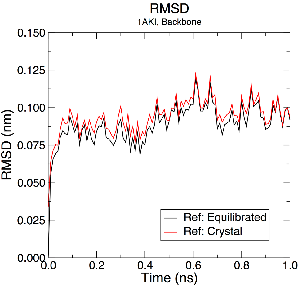

两个时间序列都显示 RMSD 水平低至 ~0.1 nm （1 Å），表明结构非常稳定。图之间的细微差异表明，t = 0 ns 处的结构与这种晶体结构略有不同。这是意料之中的，因为它已经被能量最小化，而且如前所述，位置约束并不是 100% 完美的。

回转半径

蛋白质的回转半径是其紧凑性的量度。如果蛋白质稳定折叠，它可能会保持相对稳定的 Rg 值。如果蛋白质去折叠，它的 Rg 会随着时间的推移而变化。让我们在模拟中分析溶菌酶的回转半径：

gmx gyrate -s md_0_1.tpr -f md_0_1_noPBC.xtc -o gyrate.xvg

选择第 1 组 （Protein） 进行分析：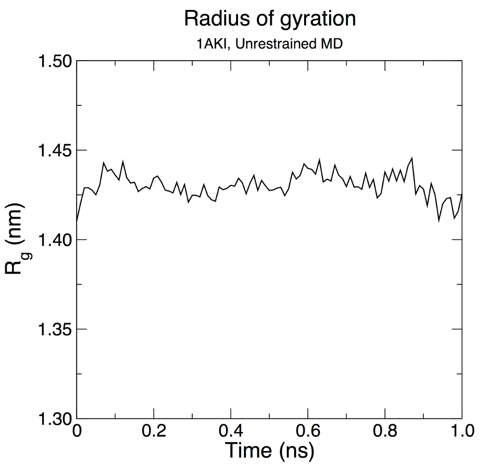

从合理不变的 Rg 值中可以看出，蛋白质在 300 K 下以紧凑（折叠）形式在 1 ns 的过程中保持非常稳定。

总结

现在，您已经使用 GROMACS 进行了分子动力学模拟，并分析了一些结果。不应将本教程视为全面。使用 GROMACS 可以进行更多类型的模拟（自由能计算、非平衡 MD 和正则模态分析，仅举几例）。您还应该查看文献和 GROMACS 手册，以调整此处提供的.mdp文件，以提高效率和准确性。